Mastering Optimization Techniques for High-Efficiency Solutions
Delve into diverse optimization methods, from 1-D to multi-dimensional approaches, emphasizing practical applications and robust strategies. Explore algorithms and trade-offs for maximum impact.

Mastering Optimization Techniques for High-Efficiency Solutions
E N D
Presentation Transcript
Optimization COS 323
Ingredients • Objective function • Variables • Constraints Find values of the variablesthat minimize or maximize the objective functionwhile satisfying the constraints
Different Kinds of Optimization Figure from: Optimization Technology Centerhttp://www-fp.mcs.anl.gov/otc/Guide/OptWeb/
Different Optimization Techniques • Algorithms have very different flavor depending on specific problem • Closed form vs. numerical vs. discrete • Local vs. global minima • Running times ranging from O(1) to NP-hard • Today: • Focus on continuous numerical methods
Optimization in 1-D • Look for analogies to bracketing in root-finding • What does it mean to bracket a minimum? (xleft, f(xleft)) (xright, f(xright)) xleft<xmid<xright f(xmid) < f(xleft) f(xmid) < f(xright) (xmid, f(xmid))
Optimization in 1-D • Once we have these properties, there is at least one local minimum between xleft and xright • Establishing bracket initially: • Given xinitial, increment • Evaluate f(xinitial), f(xinitial+increment) • If decreasing, step until find an increase • Else, step in opposite direction until find an increase • Grow increment at each step • For maximization: substitute –f for f
Optimization in 1-D • Strategy: evaluate function at some xnew (xleft, f(xleft)) (xright, f(xright)) (xnew, f(xnew)) (xmid, f(xmid))
Optimization in 1-D • Strategy: evaluate function at some xnew • Here, new “bracket” points are xnew, xmid, xright (xleft, f(xleft)) (xright, f(xright)) (xnew, f(xnew)) (xmid, f(xmid))
Optimization in 1-D • Strategy: evaluate function at some xnew • Here, new “bracket” points are xleft, xnew, xmid (xleft, f(xleft)) (xright, f(xright)) (xmid, f(xmid)) (xnew, f(xnew))
Optimization in 1-D • Unlike with root-finding, can’t always guarantee that interval will be reduced by a factor of 2 • Let’s find the optimal place for xmid, relative to left and right, that will guarantee same factor of reduction regardless of outcome
Optimization in 1-D iff(xnew) < f(xmid) new interval = else new interval = 1–2 2
Golden Section Search • To assure same interval, want = 1–2 • So, • This is the “golden ratio” = 0.618… • So, interval decreases by 30% per iteration • Linear convergence
Error Tolerance • Around minimum, derivative = 0, so • Rule of thumb: pointless to ask for more accuracy than sqrt() • Can use double precision if you want a single-precision result (and/or have single-precision data)
Faster 1-D Optimization • Trade off super-linear convergence forworse robustness • Combine with Golden Section search for safety • Usual bag of tricks: • Fit parabola through 3 points, find minimum • Compute derivatives as well as positions, fit cubic • Use second derivatives: Newton
Newton’s Method • At each step: • Requires 1st and 2nd derivatives • Quadratic convergence
Multi-Dimensional Optimization • Important in many areas • Fitting a model to measured data • Finding best design in some parameter space • Hard in general • Weird shapes: multiple extrema, saddles,curved or elongated valleys, etc. • Can’t bracket (but there are “trust region” methods) • In general, easier than rootfinding • Can always walk “downhill”
Newton’s Method inMultiple Dimensions • Replace 1st derivative with gradient,2nd derivative with Hessian
Newton’s Method inMultiple Dimensions • Replace 1st derivative with gradient,2nd derivative with Hessian • So, • Tends to be extremely fragile unless function very smooth and starting close to minimum
Steepest Descent Methods • What if you can’t / don’t want touse 2nd derivative? • “Quasi-Newton” methods estimate Hessian • Alternative: walk along (negative of) gradient… • Perform 1-D minimization along line passing through current point in the direction of the gradient • Once done, re-compute gradient, iterate
Conjugate Gradient Methods • Idea: avoid “undoing” minimization that’s already been done • Walk along direction • Polak and Ribiere formula:
Conjugate Gradient Methods • Conjugate gradient implicitly obtains information about Hessian • For quadratic function in n dimensions, gets exact solution in n steps (ignoring roundoff error) • Works well in practice…
Value-Only Methods in Multi-Dimensions • If can’t evaluate gradients, life is hard • Can use approximate (numerically evaluated) gradients:
Generic Optimization Strategies • Uniform sampling: • Cost rises exponentially with # of dimensions • Simulated annealing: • Search in random directions • Start with large steps, gradually decrease • “Annealing schedule” – how fast to cool?
Downhill Simplex Method (Nelder-Mead) • Keep track of n+1 points in n dimensions • Vertices of a simplex (triangle in 2D tetrahedron in 3D, etc.) • At each iteration: simplex can move,expand, or contract • Sometimes known as amoeba method:simplex “oozes” along the function
Downhill Simplex Method (Nelder-Mead) • Basic operation: reflection location probed byreflection step worst point(highest function value)
Downhill Simplex Method (Nelder-Mead) • If reflection resulted in best (lowest) value so far,try an expansion • Else, if reflection helped at all, keep it location probed byexpansion step
Downhill Simplex Method (Nelder-Mead) • If reflection didn’t help (reflected point still worst) try a contraction location probed bycontration step
Downhill Simplex Method (Nelder-Mead) • If all else fails shrink the simplex aroundthe best point
Downhill Simplex Method (Nelder-Mead) • Method fairly efficient at each iteration(typically 1-2 function evaluations) • Can take lots of iterations • Somewhat flakey – sometimes needs restart after simplex collapses on itself, etc. • Benefits: simple to implement, doesn’t need derivative, doesn’t care about function smoothness, etc.
Rosenbrock’s Function • Designed specifically for testingoptimization techniques • Curved, narrow valley
Constrained Optimization • Equality constraints: optimize f(x)subject to gi(x)=0 • Method of Lagrange multipliers: convert to a higher-dimensional problem • Minimize w.r.t.
Constrained Optimization • Inequality constraints are harder… • If objective function and constraints all linear, this is “linear programming” • Observation: minimum must lie at corner of region formed by constraints • Simplex method: move from vertex to vertex, minimizing objective function
Constrained Optimization • General “nonlinear programming” hard • Algorithms for special cases (e.g. quadratic)
Global Optimization • In general, can’t guarantee that you’ve found global (rather than local) minimum • Some heuristics: • Multi-start: try local optimization fromseveral starting positions • Very slow simulated annealing • Use analytical methods (or graphing) to determine behavior, guide methods to correct neighborhoods


