Download
1 / 71
750 likes | 1.24k Vues
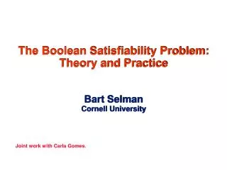
The Boolean Satisfiability Problem: Theory and Practice Bart Selman Cornell University. Joint work with Carla Gomes. The Quest for Machine Reasoning. Objective: Develop foundations, technology, and tools to enable effective practical machine reasoning. Machine Reasoning (1960-90s).

E N D
The Boolean Satisfiability Problem:Theory and PracticeBart Selman Cornell University Joint work with Carla Gomes.
The Quest for Machine Reasoning Objective: Develop foundations, technology, and tools to enable effective practical machine reasoning. Machine Reasoning (1960-90s) Current reasoning technology Revisiting the challenge: Significant progress with new ideas / tools for dealing with complexity (scale-up), uncertainty, and multi-agent reasoning. Computational complexity of reasoning appearsto severly limit real-world applications.
Fundamental challenge: Combinatorial Search Spaces • Significant progress in the last decade. • How much? • For propositional reasoning: • -- We went from 100 variables, 200 clauses (early 90’s) • to 1,000,000 vars. and 5,000,000 constraints in • 10 years. Search space: from 10^30 to 10^300,000. • -- Applications: Hardware and Software Verification, • Test pattern generation, Planning, Protocol Design, • Routers, Timetabling, E-Commerce (combinatorial • auctions), etc.
How can deal with such large combinatorial spaces and • still do a decent job? • I’ll discuss recent formal insights into • combinatorial search spaces and their • practical implications that makes searching • such ultra-large spaces possible. • Brings together ideas from physics of disordered systems • (spin glasses), combinatorics of random structures, and • algorithms. • But first, what is BIG?
What is BIG? Consider a real-world Boolean Satisfiability (SAT) problem I.e., ((not x_1) or x_7) ((not x_1) or x_6) etc. x_1, x_2, x_3, etc. our Boolean variables (set to True or False) Set x_1 to False ??
10 pages later: … I.e., (x_177 or x_169 or x_161 or x_153 … x_33 or x_25 or x_17 or x_9 or x_1 or (not x_185)) clauses / constraints are getting more interesting… Note x_1 …
Finally, 15,000 pages later: HOW? Combinatorial search space of truth assignments: Current SAT solvers solve this instance in approx. 1 minute!
Progress SAT Solvers Source: Marques Silva 2002
From academically interesting to practically relevant. • We now have regular SAT solver competitions. • Germany ’89, Dimacs ’93, China ’96, SAT-02, SAT-03, SAT-04, SAT05. • E.g. at SAT-2004 (Vancouver, May 04): • --- 35+ solvers submitted • --- 500+ industrial benchmarks • --- 50,000+ instances available on the WWW.
DARPA Research Program Real-World ReasoningTackling inherent computational complexity 1M 5M Multi-Agent Systems 10301,020 0.5M 1M Hardware/Software Verification 10150,500 Worst Case complexity Exponential Complexity 200K 600K Military Logistics 1015,050 50K 200K Chess 103010 No. of atoms on earth 10K 50K Deep space mission control Technology Targets 1047 • High-Performance Reasoning • Temporal/ uncertainty reasoning • Strategic reasoning/Multi-player Seconds until heat death of sun 100 200 Car repair diagnosis 1030 Protein folding calculation (petaflop-year) Variables 100 10K 20K 100K 1M Rules (Constraints) Example domains cast in propositional reasoning system (variables, rules).
A Journey from Random to Structured Instances • I --- Random Instances • --- phase transitions and algorithms • --- from physics to computer science • II --- Capturing Problem Structure • --- problem mixtures (tractable / intractable) • --- backdoor variables, restarts, and heavy tails • III --- Beyond Satisfaction • --- sampling, counting, and probabilities • --- quantification
Part I) ---- Random Instances • Easy-Hard-Easy patterns (computational) and • SAT/UNSAT phase transitions (“structural”). • Their study provides an interplay of work from • statistical physics, computer science, and • combinatorics. • We’ll briefly consider “The State of Random 3-SAT”.
Phase transition Random Walk DP DP’ GSAT Walksat SP Random 3-SAT as of 2005 Linear time algs. Mitchell, Selman, and Levesque ’92
Linear time results --- Random 3-SAT • Random walk up to ratio 1.36 (Alekhnovich and Ben Sasson 03). • empirically up to 2.5 • Davis Putnam (DP) up to 3.42 (Kaporis et al. ’02) empirically up to 3.6 • exponential, ratio 4.0 and up (Achlioptas and Beame ’02) • approx. 400 vars at phase transition • GSAT up till ratio 3.92 (Selman et al. ’92, Zecchina et al. ‘02) • approx. 1,000 vars at phase transition • Walksat up till ratio 4.1 (empirical, Selman et al. ’93) • approx. 100,000 vars at phase transition • Survey propagation (SP) up till 4.2 • (empirical, Mezard, Parisi, Zecchina ’02) • approx. 1,000,000 vars near phase transition • Unsat phase: little algorithmic progress. • Exponential resolution lower-bound (Chvatal and Szemeredi 1988)
Linear time results --- Random 3-SAT • Random walk up to ratio 1.36 (Alekhnovich and Ben Sasson 03). • empirically up to 2.5 • Davis Putnam (DP) up to 3.42 (Kaporis et al. ’02) empirically up to 3.6 • exponential, ratio 4.0 and up (Achlioptas and Beame ’02) • approx. 400 vars at phase transition • GSAT up till ratio 3.92 (Selman et al. ’92, Zecchina et al. ‘02) • approx. 1,000 vars at phase transition • Walksat up till ratio 4.1 (empirical, Selman et al. ’93) • approx. 100,000 vars at phase transition • Survey propagation (SP) up till 4.2 • (empirical, Mezard, Parisi, Zecchina ’02) • approx. 1,000,000 vars near phase transition • Unsat phase: little algorithmic progress. • Exponential resolution lower-bound (Chvatal and Szemeredi 1988)
Linear time results --- Random 3-SAT • Random walk up to ratio 1.36 (Alekhnovich and Ben Sasson 03). • empirically up to 2.5 • Davis Putnam (DP) up to 3.42 (Kaporis et al. ’02) empirically up to 3.6 • exponential, ratio 4.0 and up (Achlioptas and Beame ’02) • approx. 400 vars at phase transition • GSAT up till ratio 3.92 (Selman et al. ’92, Zecchina et al. ‘02) • approx. 1,000 vars at phase transition • Walksat up till ratio 4.1 (empirical, Selman et al. ’93) • approx. 100,000 vars at phase transition • Survey propagation (SP) up till 4.2 • (empirical, Mezard, Parisi, Zecchina ’02) • approx. 1,000,000 vars near phase transition • Unsat phase: little algorithmic progress. • Exponential resolution lower-bound (Chvatal and Szemeredi 1988)
Linear time results --- Random 3-SAT • Random walk up to ratio 1.36 (Alekhnovich and Ben Sasson 03). • empirically up to 2.5 • Davis Putnam (DP) up to 3.42 (Kaporis et al. ’02) empirically up to 3.6 • exponential, ratio 4.0 and up (Achlioptas and Beame ’02) • approx. 400 vars at phase transition • GSAT up till ratio 3.92 (Selman et al. ’92, Zecchina et al. ‘02) • approx. 1,000 vars at phase transition • Walksat up till ratio 4.1 (empirical, Selman et al. ’93) • approx. 100,000 vars at phase transition • Survey propagation (SP) up till 4.2 • (empirical, Mezard, Parisi, Zecchina ’02) • approx. 1,000,000 vars near phase transition • Unsat phase: little algorithmic progress. • Exponential resolution lower-bound (Chvatal and Szemeredi 1988)
5.19 5.081 4.762 4.596 4.506 4.601 4.643 Random Walk DP DP’ GSAT Walksat SP Random 3-SAT as of 2004 Linear time algs. Upper bounds by combinatorial arguments (’92 – ’05)
Exact Location of Threshold • Surprisingly challenging problem ... • Current rigorously proved results: • 3SAT threshold lies between 3.42 and 4.506. • Motwani et al. 1994; Broder et al. 1992; • Frieze and Suen 1996; Dubois 1990, 1997; • Kirousis et al. 1995; Friedgut1997; • Archlioptas et al. 1999; • Beame, Karp, Pitassi, and Saks 1998; • Impagliazzo and Paturi 1999; Bollobas, • Borgs, Chayes, Han Kim, and • Wilson1999; Achlioptas, Beame and • Molloy 2001; Frieze 2001; Zecchina et al. 2002; • Kirousis et al. 2004; Gomes and Selman, Nature ’05; • Achlioptaset al.Nature ’05; and ongoing… Empirical: 4.25 --- Mitchell, Selman, and Levesque ’92, Crawford ’93.
From Physics to Computer Science • Exploits correspondence between SAT and physical systems with many interacting particles. Satisfied iff [(x_i = 1 and x_j =1) OR (x_i =0 and x_j=0)] Basic model for magnetism: The Ising model (Ising ’24). Spins are “trying to align themselves”. But system can be “frustrated” some pairs want to align; some want to point in the opposite direction of each other.
We can now assign a probability distribution over the assignments/ • states --- the Boltzmann distribution: • Prob(S) = 1/Z * exp(- E(S) / kT) • where, • E is the “energy” = # unsatisfied constraints, • T is the “temperature” a control parameter, • k is the Boltzmann constant, and • Z is the “partition function” (normalizes). • Distribution has a physical interpretation (captures thermodynamic • equilibrium) but, for us, key property: • With T 0, only minimum energy states have non-zero • probability. So, by taking T 0, we can find properties of the • satisfying assignments of the SAT problem.
In fact, partition function Z, contains all necessary information. Z =∑ exp (- E(S)/kT) sum is over all 2N possible states / (truth) assignments. Are we really making progress here?? Sum over an exponential number of terms, 2N... in CS, N ~ 106 in physics, N ~ 1023 Fortunately, physicists have been studying “Z” for 100+ years. (Feynman Lectures: “Statistical physics = study of Z”.) They have developed a powerful set of analytical tools to calculate / approximate Z : e.g. mean field approximations, Monte Carlo methods, matrix transfer methods, renormalization techniques, replica methods and cavity methods.
Physics contributing to computation • 80’s --- Simulated annealing • General combinatorial search technique, inspired by physics. • (Kirkpatrick et al., Science ’83) • 90’s --- Phase transitions in computational systems • Discovery of physical laws and phenomena (e.g. 1st and 2nd • order transitions) in computational systems. • (Cheeseman et al. ’91; Selman et al. ’92; • Explicit connection to physics: • Kirkpatrick and Selman, Science ’94 (finite-size scaling); • Monasson et al., Nature ’99. (order of phase transition)) • ’02 --- Survey Propagation • Analytical tool from statistical physics leads to powerful • algorithmic method. 1 million var wffs. (Mezard et al., Science ’02). • More expected!
A Journey from Random to Structured Instances • I --- Random Instances • --- phase transitions and algorithms • --- from physics to computer science • II --- Capturing Problem Structure • --- problem mixtures (tractable / intractable) • --- backdoor variables, restarts, and heavy-tails • III --- Beyond Satisfaction • --- sampling, counting, and probabilities • --- quantification
Part II) --- Capturing Problem Structure • Results and algorithms for hard random k-SAT • problems have had significant impact on • development of practical SAT solvers. However… • Next challenge: Dealing with SAT problems with • more inherent structure. • Topics (with lots of room for further analysis): • Mixtures of tractable/intractable stucture • Backdoor variables and heavy tails
II A) Mixtures: The 2+p-SAT problem • Motivation: Most real-world computational • problems involve some mix of tractable • and intractable sub-problems. • Study: mixture of binary and ternary clauses • p = fraction ternary • p = 0.0 --- 2-SAT / p = 1.0 --- 3-SAT • What happens in between?
Phase transitions (as expected…) • Computational properties (surprise…) • (Monasson, Zecchina, Kirkpatrick, Selman, Troyansky 1999.)
Phase Transition for 2+p-SAT We have good approximations for location of thresholds.
Computational Cost: 2+p-SATTractable substructure can dominate! > 40% 3-SAT --- exponential scaling Mixing 2-SAT (tractable) & 3-SAT (intractable) clauses. Medium cost <= 40% 3-SAT --- linear scaling Num variables (Monasson et al. 99; Achlioptas ‘00)
Results for 2+p-SAT • p < = 0.4 --- model behaves as 2-SAT • search proc. “sees” only binary constraints • smooth, continuous phase transition (2nd order) • p > 0.4 --- behaves as 3-SAT (exponential scaling) • abrupt, discontinuous transition (1st order) • Note: problem is NP-complete for any p > 0. Conjecture: abrupt phase transition implies exponential search cost.
Lesson learned • In a worst-case intractable problem --- such • as 2+p-SAT --- having a sufficient amount of • tractable problem substructure (possibly • hidden) can lead to provably poly-time average • case behavior. • Next: • Capturing hidden problem structure. • (Gomes et al. 03, 04)
II B) --- Backdoors to the real-world Observation: Complete backtrack style search SAT solvers (e.g. DPLL) display a remarkably wide range of run times. Even when repeatedly solving the same problem instance; variable branching is choice randomized. Run time distributions are often “heavy-tailed”. Orders of magnitude difference in run time on different runs. (Gomes et al. 1998; 2000)
Heavy-tails on structured problems 50% runs: solved with 1 backtrack 10% runs: > 100,000 backtracks Unsolved fraction 1 100,000 Number backtracks (log)
Randomized Restarts • Solution: randomize the backtrack strategy • Add noise to the heuristic branching (variable choice) function • Cutoff and restart search after a fixed number of backtracks • Provably Eliminates heavy tails • In practice: rapid restarts with low cutoff can dramatically improve performance • (Gomes et al. 1998, 1999) • Exploited in current SAT solvers combined • with clause learning and non-chronological backtracking. • (Chaff etc.)
3 R Logistics Planning 108 mins. 95 sec. Scheduling 14 411 sec 250 sec Scheduling 16 ---(*) 1.4 hours Circuit Synthesis 2 Circuit Synthesis 1 ---(*) ---(*) 17min. 165sec. ---(*) ~18 hrs Scheduling 18 Sample Results Random Restarts Deterministic (*) not found after 2 days
Formal Model Yielding Heavy-Tailed Behavior • T - the number of leaf nodes visited up to and including the successful node; b - branching factor (heavy-tailed distribution) p = probability wrong branching choice. 2^k time to recover from k wrong choices. b = 2 (Chen, Gomes, and Selman ’01; Williams, Gomes, and Selman‘03)
Intuitively: Exponential penalties hidden in backtrack search, consisting of large inconsistent subtrees in the search space. But, for restarts to be effective, you also need short runs. Where do short runs come from?
Explaining short runs:Backdoors to tractability • Informally: • A backdoor to a given problem is a subset of the variables such • that once they are assigned values, the polynomial propagation • mechanism of the SAT solver solves the remaining formula. • Formal definition includes the notion of a “subsolver”: • a polynomial simplification procedure with certain general • characteristics found in current DPLL SAT solvers. Backdoors correspond to “clever reasoning shortcuts” in the search space.
Backdoors (wrt subsolver A; SAT case): Strong backdoors (wrt subsolver A; UNSAT case): Note: Notion of backdoor is related to but different from constraint-graph based notions such as cutsets. (Dechter 1990; 2000)
Backdoors can be surprisingly small: Most recent: Other combinatorial domains. E.g. graphplan planning, near constant size backdoors (2 or 3 variables) and log(n) size in certain domains. (Hoffmann, Gomes, Selman ’05) Backdoors capture critical problem resources (bottlenecks).
Backdoors --- “seeing is believing” Constraint graph of reasoning problem. One node per variable: edge between two variables if they share a constraint. Logistics_b.cnf planning formula. 843 vars, 7,301 clauses, approx min backdoor 16 (backdoor set = reasoning shortcut) Visualization by Anand Kapur.
After setting just 12 (out of 800+) backdoor vars– problem almost solved.
Another example MAP-6-7.cnf infeasible planning instances. Strong backdoor of size 3. 392 vars, 2,578 clauses.
After setting 2 (out of 392) backdoor vars. --- reducing problem complexity in just a few steps!
Last example. Inductive inference problem --- ii16a1.cnf. 1650 vars, 19,368 clauses. Backdoor size 40.
Some other intermediate stages: After setting 38 (out of 1600+) backdoor vars: So: Real-world structure hidden in the network. Can be exploited by automated reasoning engines.
But… we also need to take into account the • cost of finding the backdoor! • We considered: • Generalized Iterative Deepening • Randomized Generalized Iterative Deepening • Variable and value selection heuristics • (as in current solvers)