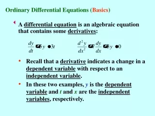
Ordinary Differential Equations
ODE. Ordinary Differential Equations. 一阶常微分方程的初值问题: 节点: x 1 <x 2 < … <x n 步长 为常数. 一 欧拉方法(折线法) y i +1 = y i + h f ( x i , y i ) ( i =0,1, … , n- 1) 优点:计算简单。 缺点:一阶精度。 二 改进的欧拉方法. 改进的欧拉公式可改写为 它每一步计算 f ( x,y ) 两次,截断误差为 O( h 3 ). 精确解 :.


Ordinary Differential Equations
E N D
Presentation Transcript
ODE Ordinary Differential Equations
一阶常微分方程的初值问题: • 节点:x1<x2< … <xn • 步长 为常数
一 欧拉方法(折线法) yi+1=yi+h f(xi,yi) (i =0,1, …, n-1) 优点:计算简单。 缺点:一阶精度。 • 二 改进的欧拉方法
改进的欧拉公式可改写为 它每一步计算f(x,y)两次,截断误差为O(h3)
精确解: function [t,y] = Heun(ode,tspan,h,y0) t = (tspan(1):h:tspan(end))'; n = length(t); y = y0*ones(n,1); for i=2:n k1 = feval(ode,t(i-1),y(i-1)); k2 = feval(ode,t(i),y(i-1)+h*k1); y(i) = y(i-1)+h*(k1+k2)/2; end
三 龙格—库塔法(Runge-Kutta) 欧拉公式可改写为 它每一步计算 f (xi,yi) 一次,截断误差为O(h2)
标准四阶龙格—库塔公式 每一步计算 f (x, y) 四次,截断误差为O(h5)
对于两个分量的一阶常微分方程组 用经典4阶 Runge-Kutta 法求解的格式为
n级显式Runge-Kutta 方法的一般计算格式: 其中 Adams 外插公式(Adams-Bashforth 公式)是一类 k+1 步 k+1 阶显式方法 三步法(k=2), 四步法(k=3), Adams 内插公式(Adams-Moulton 公式)是一类 k+1 步 k+2 阶隐式方法 三步法(k=2), Adams 预估-校正方法(Adams-Bashforth-Moulton 公式) 一般取四步外插法与三步内插法结合。
#include <stdio.h> #include <stdlib.h> #include <math.h> #define TRUE 1 main() { int nstep_pr, j, k; float h, hh, k1, k2, k3, k4, t_old, t_limit, t_mid, t_new, t_pr, y, ya, yn; double fun(); printf( "\n Fourth-Order Runge-Kutta Scheme \n" ); while(TRUE){ printf( "Interval of t for printing ?\n" ); scanf( "%f", &t_pr ); printf( "Number of steps in one printing interval?\n" ); scanf( "%d", &nstep_pr ); printf( "Maximum t?\n" ); scanf( "%f", &t_limit ); y = 1.0; /* Setting the initial value of the solution */ h = t_pr/nstep_pr; printf( "h=%g \n", h ); t_new = 0; /* Time is initialized. */ hh = h/2; printf( "--------------------------------------\n" ); printf( " t y\n" ); printf( "--------------------------------------\n" ); printf( " %12.5f %15.6e \n", t_new, y );
do{ for( j = 1; j <= nstep_pr; j++ ){ t_old = t_new; t_new = t_new + h; yn = y; t_mid = t_old + hh; yn = y; k1 = h*fun( yn, t_old ); ya = yn + k1/2; k2 = h*fun( ya, t_mid ); ya = yn + k2/2; k3 = h*fun( ya, t_mid ); ya = yn + k3 ; k4 = h*fun( ya, t_new ); y = yn + (k1 + k2*2 + k3*2 + k4)/6; } printf( " %12.5f %15.6e \n", t_new, y ); } while( t_new <= t_limit ); printf( "--------------------------------------\n" ); printf( " Maximum t limit exceeded \n" ); printf( "Type 1 to continue, or 0 to stop.\n" ); scanf( "%d", &k ); if( k != 1 ) exit(0); } } double fun(y, t) float y, t; { float fun_v; fun_v = -y; return( fun_v ); }
四 误差的控制 我们常用事后估计法来估计误差,即从xi出发,用两种办法计算y(xi+1)的近似值。 记 为从xi出发以h为步长得到的y(xi+1)的 近似值,记 为从xi出发以 h/2 为步长跨 两步得到的y(xi+1)的近似值。设给定精度为ε。如果不等式 成立,则 即为y(xi+1)的满足精度要求的近似值。
自适应: 使用2个不同的h。如果一个大的h和一个小的h得到的解相同,那么减小h就没有意义了;相反如果两个解差别大,可以假设大h值得到的解是不精确的。 使用相同的h值,2种不同的算法。如果低精度算法与高精度算法的结果相同,则没有必要减小h。
Matlab 函数 Ode23 非刚性, 单步法, 二三阶Runge-Kutta,精度低 Ode45非刚性, 单步法, 四五阶Runge-Kutta,精度较高,最常用 Ode113非刚性, 多步法, 采用可变阶(1-13)Adams PECE 算法, 精度可高可低 Ode15s 刚性, 多步法,采用Gear’s (或BDF)算法, 精度中等. 如果ode45很慢, 系统可能是刚性的,可试此法 Ode23s 刚性, 单步法, 采用2阶Rosenbrock法, 精度较低, 可解决ode15s 效果不好的刚性方程. Ode23t 适度刚性, 采用梯形法则,适用于轻微刚性系统,给出的解无数值衰减. Ode23tb 刚性, TR-BDF2, 即R-K的第一级用梯形法则,第二级用Gear 法. 精度较低, 对于误差允许范围比较差的情况,比ode15s好.
Matlab’s ode23 (Bogacki, Shampine)
Runge-Kutta-Fehlberg方法(RKF45) 4阶Runge-Kutta近似 5阶Runge-Kutta近似 局部误差估计 Matlab’s ode45 is a variation of RKF45
Van der Pol: function xdot = vdpol(t,x) xdot(1) = x(2); xdot(2) = -(x(1)^2 -1)*x(2) -x(1); xdot = xdot'; % VDPOL must return a column vector. % xdot = [x(2); -(x(1)^2 -1)*x(2) -x(1)]; % xdot = [0 , 1; -1 ,-(x(1)^2 -1)] *x; t0 = 0; tf = 20; x0 = [0; 0.25]; [t,x] = ode45(@vdpol,[t0,tf],x0); plot(t,x); figure(101) plot(x(:,1),x(:,2));
Lorenz吸引子 function xdot = lorenz(t,x) xdot = [ -8/3, 0, x(2); 0, -10, 10; -x(2), 28, -1]*x; x0 = [0,0,eps]'; [t,x] = ode23('lorenz',[0,100],x0); plot3(x(:,1),x(:,2),x(:,3)); plot(x(:,1),x(:,2));
刚性方程 向后差分方法(Gear’s method) 隐式Runge-Kutta法 function yp = examstiff(t,y) yp = [-2, 1; 998, -998]*y + [2*sin(t);999*(cos(t)-sin(t))]; y0 = [2;3]; tic,[t,y] = ode113('examstiff',[0,10],y0);toc tic,[t,y] = ode45('examstiff',[0,10],y0);toc tic,[t,y] = ode23('examstiff',[0,10],y0);toc tic,[t,y] = ode23s('examstiff',[0,10],y0);toc tic,[t,y] = ode15s('examstiff',[0,10],y0);toc tic,[t,y] = ode23t('examstiff',[0,10],y0);toc tic,[t,y] = ode23tb('examstiff',[0,10],y0);toc
初值为 时, 解析解为 线性隐式ODE: 完全隐式ODE(Matlab7): Weissinger方程: function f = weissinger(t,y,yp) f = t*y^2*yp^3 - y^3*yp^2 + t*(t^2+1)*yp - t^2*y; t0 = 1; y0 = sqrt(3/2); yp0= 0; % guess [y0,yp0] = decic(@weissinger,t0,y0,1,yp0,0); % 求出自洽初值。保持y0不变 [t,y] = ode15i(@weissinger,[1,10],y0,yp0); ytrue = sqrt(t.^2+0.5); plot(t,ytrue,t,y,'o')
function yp = ddefun(t,y,Z) yp = zeros(2,1); % define lags=[1,3] yp(1) = Z(1,2)^2 + Z(2,1)^2; yp(2) = y(1) + Z(2,1); function y = ddehist(t) y = zeros(2,1); y(1) = 1; y(2) = t-2; 延迟微分方程 Sol = dde23(ddefun,lags,ddehist,tspan) lags = [1,3]; sol = dde23(@ddefun,lags,@ddehist,[0,1]); hold on; plot(sol.x,sol.y(1,:),'b-'); plot(sol.x,sol.y(2,:),'r-'); 初值:
有限差分法 二阶线性边值问题 差分离散: bvp4c
线性边值问题的打靶法: 二阶线性边值问题(11)的可以通过求解下面两个初值问题获得。 (IVP1) (IVP2) 原来边值问题的解可以表示为: 非线性边值问题的打靶法
符号计算 y = dsolve('D2y = -a^2*y','x') %求通解 y = dsolve('D2y = -a^2*y','y(0)=1','Dy(pi/a)=0','x') [x,y] = dsolve('Dx=4x-2y','Dy=2x-y','t') Pdetool 求解区域,定义边界,网格划分,计算,画图,保存文件求解 边条 解析解 演示求解过程
Stokes 问题 Q1-P0有限元离散
前台阶流(A Mach 3 Wind Tunnel with a Step) 模拟放置在风洞中的前台阶流动。风洞尺寸:宽1.0,长3.0,台阶高0.2,放置在距风洞左边界0.6个单位长度处。 物理问题的控制方程:
Sod问题 Sod问题是在激波管中充以两种介质,维持一定的压力差,用隔膜分开;当隔膜突然破裂后,形成间断面,研究其时间发展情况。 Euler方程组:
A picture is worth a thousand words. - Anonymous Make it right before you make it faster. - Brain W. Kernighan, P. J. Plauger, The Elements of Programming Style(1978)