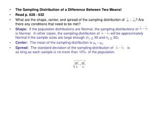
Significance of the Difference Between Two Sample Means
400 likes | 641 Vues
Significance of the Difference Between Two Sample Means. Previously…. We learned how to test the hypothesis that one sample came from a population that we have information about, either parameters (like a known μ ) or claims (like a claimed μ ). H 0 : μ = μ 0

Significance of the Difference Between Two Sample Means
E N D
Presentation Transcript
Previously… • We learned how to test the hypothesis that one sample came from a population that we have information about, either parameters (like a known μ) or claims (like a claimed μ). • H0: μ = μ0 • We knew what μ was (it was a constant), so we could just plug it into our formula and determine ourtscore. • We used the sampling distribution of means as our reference distribution.
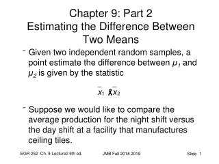
Two-sample ttest • We are going to learn how to compare two samples, one control group and one treatment group. • We will treat the control group as the population and the treatment group as our single sample.
Draw Two Samples and Compare (Unknown) Population Control Treatment
Our Hypothesis • H0: μ1 = μ2 • Instead of using to estimate the significance of our treatment, we will use .
Independent Samples • Independent just means that one group cannot influence the outcome of the other group. • If we randomly sample from the population and randomly assign individuals to each group, we generally won’t have a problem.
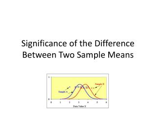
Sampling Distribution of the Mean Differences • Because we are dealing with two samples and we assume that they are being drawn from the same population (remember our null hypothesis), the reference distribution we will use is the distribution of the differences between all pairs of sample means.
Draw two samples: (Unknown) Population Control Treatment
Then find the difference between their means: − − Repeat − − − −
Sampling Distribution of the Mean Differences • If you plot the mean differences on a frequency distribution, the differences will vary around the “true difference.” • The differences will be normally distributed (perfectly so with an infinite number of mean differences).
If H0 is True • You will find that the mean of the mean differences is 0. • In other words, the true difference is 0 (there is no difference). • Therefore, the control group and sample group “come from the same population,” which means that they do not differ with respect to the variable you are measuring.
If H0 is False • You will find that the mean of the mean differences is not 0. • In other words, the true difference is not equal to 0 (there is a difference). • Therefore, the control group and treatment group come from different populations, which means that they do differ with respect to the variable you are measuring.
Properties • Here is a fancy way of saying what we just said (the mean of all sample differences is equal to the difference between the population means): • The larger the sample sizes, the closer the curve will be to the normal curve. • The larger the sample sizes, the smaller the standard deviation of sampling distribution differences.
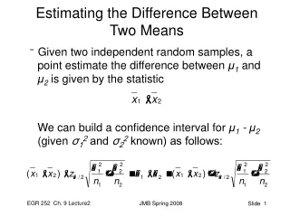
Standard Error of the Difference • The standard deviation of the mean differences is called the standard error of the difference between means and is defined mathematically as follows:
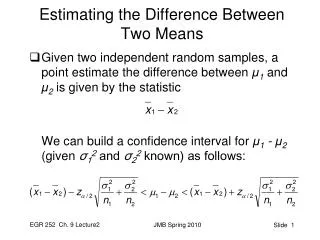
Back to Reality • This is all theoretical, since you won’t be drawing an infinite number of samples and comparing their means, and you won’t know the population parameters. • So what do we do with our two samples?
Estimated Standard Error of the Difference • The estimated standard error of the difference formula is the same, but with statistics substituted for the parameters:
Estimated Standard Error of the Difference • The formula that we will be using for calculation can be used on samples of different sizes (which is why we will use it): • Notice that you know all of the necessary terms. • The reason it looks complex is that the variance is “weighted” by sample size. Larger samples get more say in determining the standard error of the difference.
Finding the tscore • Remember in the last unit, we found the tscore using a formula very similar to the z score formula. We are going to do the same thing here. • If we knew the population parameters, we would use this formula
Finding the t score • Of course, we don’t know the population parameters, so we use this formula instead: • And since we are assuming that the samples come from the same population (μ1– μ2 = 0), we can write it this way:
Computing t • If we substitute the computational formula for the estimated standard error of the difference in the denominator, we get this monster formula: • But notice that it’s all stuff we’ve done before.
Using the ttable • Once we have the tscore, we can check the ttable to see if the difference between our samples is “significant.” • Just as before if our tobt (the value we get from our formula) is LARGER than our tcrit (the value we find in the table), we reject the null. • One important difference: for our df we use N1 + N2 – 2.
Activity #1 • An educational experiment with participants randomly sampled and assigned to two groups: traditional lecture and group discussion produces the following results. • Lecture Group: N = 25, Mean = 81.7, s = 8.3 • Discussion Group: N = 25, Mean = 74.1, s= 10.1 • Is there a “significant” difference between the two groups at the α = .05 level? At the α = .01 level?
Step 1 • State the H0: μ1 = μ2 • In other words, there is no difference between the two groups (i.e., they came from the same population). • Choose an α level (we will look at both values, just for fun).
Step 2 • State your rejection rule: • Reject H0 if |tobt| ≥ tcrit • using df = N1 + N2 – 2 = 25 + 25 – 2 = 48 (we will use 50 in our table), tcrit = 2.0086 (5%) and 2.6778 (1%)
Step 3 • Now we compute:
Step 4 • Make a decision: • We know that tcrit = 2.0086 (5%) and 2.6778 (1%) • We know that tobt = 2.906 • We can see that tobt is greater than both tcrit values, so we would reject the null regardless of the α level we had chosen.
Step 5 • Interpret your results: • The difference between the lecture group and the discussion group was statistically significant, t= 2.906, p < .01. • Make sure you know what this means: the probability of obtaining samples with differences this great or greater if the null hypothesis is true (there is no difference between the groups) is less than .01.
Assumptions of the Independent Two-Sample t Test • Normal distribution: we assume that the DV in the populations are normally distributed. • Homogeneity of Variance: (homogeneity = sameness) we assume that the population variances are the same. • Independent Samples: we assume that the samples are independent
Violations of the Assumption • If any one of the assumptions is violated, the t test will often continue to produce valid results. The test is robust.
However • If homogeneity of variance is violated (i.e., the variances are dissimilar) AND the sample sizes are different, you could get wacky results. • Also, if the third assumption, independence, is violated, you will want to use a different test.
Dependent Samples • If the samples are not independent, they are dependent. • Actually, using dependent samples can increase the power of your analysis, which is a good thing (it means you have a greater chance of rejecting the null if there is a difference between the samples).
Matched Pairs • Finding subjects that are alike with regard to a variable that is likely to influence the experimental outcome and assigning one to each group (e.g., matching people with similar IQ scores for an academic experiment). • To conduct a matched pairs experiment, you need information about at least one additional variable (like IQ score, bench press maximum, relation to other subjects, etc.)
Within-subject Comparisons(Repeated Measures Design) • Each subject is exposed to both treatment and control conditions. • The order of exposure is randomized and counterbalanced. • You can get away with smaller sample sizes.
Why More Power? • If the subjects are matched, the difference between means will be closer to the actual difference and not as heavily influenced by variation caused by the “matching variable.” • With repeated measures, the subjects are the same in both groups, so you have even less uncontrolled variance.
Computing t for Dependent Samples • First, construct a table with each pair (matched pairs) or individual (repeated measures) in one row.
Computing t for Dependent Samples • Calculate the difference (D) between each condition for each row. Then square D.
Computing t for Dependent Samples • Find the mean of the differences: • Find the estimated standard error the difference:
Computing t for Dependent Samples • Calculate t:
Finding tcrit • Finding the critical value is the same as before, except for an important difference: • When finding tcrit use the number of pairs (for matched pairs) or individuals (for repeated measures) as N. df = N – 1.
Homework • Study for Chapter 10 Quiz • Read Chapter 11 • Do Chapter 10 HW