Accelerating Spatially Varying Gaussian Filters
430 likes | 631 Vues
Accelerating Spatially Varying Gaussian Filters. Jongmin Baek and David E. Jacobs Stanford University. Motivation. Input. Spatially Varying Gaussian Filter. Gaussian Filter. Roadmap. Accelerating Spatially Varying Gaussian Filters Accelerating Spatially Varying Gaussian Filters

Accelerating Spatially Varying Gaussian Filters
E N D
Presentation Transcript
Accelerating Spatially Varying Gaussian Filters Jongmin Baek and David E. Jacobs Stanford University
Motivation Input Spatially Varying Gaussian Filter Gaussian Filter
Roadmap • Accelerating Spatially VaryingGaussian Filters • AcceleratingSpatially Varying Gaussian Filters • AcceleratingSpatially Varying Gaussian Filters • Applications
Gaussian Filters Position Value • Given pairs as input,
Gaussian Filters • Each output value …
Gaussian Filters • … is a weighted sum of input values …
Gaussian Filters • … whose weight is a Gaussian …
Gaussian Filters • … in the space of the associated positions.
Gaussian Filters: Uses Gaussian Blur
Gaussian Filters: Uses Bilateral Filter
Gaussian Filters: Uses Non-local Means Filter
Gaussian Filters: Summary • Applications • Denoisingimages and meshes • Data fusion and upsampling • Abstraction / Stylization • Tone-mapping • ... • Previous work on fast Gaussian Filters • Bilateral Grid (Chen, Paris, Durand; 2007) • Gaussian KD-Tree (Adams et al.; 2009) • Permutohedral Lattice (Adams, Baek, Davis; 2010)
Gaussian Filters: Implementations Summary of Previous Implementations: • A separable blur flanked by resampling operations. • Exploit the separability of the Gaussian kernel.
Spatially Varying Gaussian Filters Spatially Invariant Spatially varying covariance matrix
Spatial Variance in Previous Work • Trilateral Filter (Choudhury and Tumblin, 2003) • Tilt the kernel of a bilateral filter along the image gradient. • “Piecewise linear”instead of“Piecewise constant”model.
Spatially Varying Gaussian Filters: Tradeoff Input Bilateral-filtered Trilateral-filtered Benefits: • Can adapt the kernel spatially. • Better filtering performance. • Cost: • No longer separable. • No existing acceleration schemes.
Acceleration Problem: • Spatially varying (thus non-separable) Gaussian filter • Existing Tool: • Fast algorithms for spatially invariant Gaussian filters • Solution: • Re-formulate the problem to fit the tool. • Need to obey the “piecewise-constant” assumption
Naïve Approach (Toy Example) I LOST THE GAME Input Signal 1 2 1 3 1 4 Desired Kernel filtered w/ 1 1 1 1 filtered w/ 2 2 filtered w/ 3 3 Output Signal filtered w/ 4 4
Challenge #1 • In practice, the # of kernels can be very large. Desired Kernel K(x) Range of Kernels needed Pixel Location x
Solution #1 • Sample a few kernels and interpolate. Desired Kernel K(x) K1 Interpolate result! K2 Sampled kernels K3 Pixel Location x
Assumptions Interpolation needs an extra assumption to work: • The covariance matrix Ʃi is either piecewise-constant, or smoothly varying. • Kernel is spatially varying, but locally spatially invariant.
Challenge #2 • Runtime scales with the # of sampled kernels. Desired Kernel K(x) K1 Filter only some regions of the image with each kernel. (“support”) K2 Sampled kernels K3 Pixel Location x
Defining the Support In this example, x needs to be in the support of K1&K2. Desired Kernel K(x) K1 K2 K3 Pixel Location x
Dilating the Support Desired Kernel K(x) K1 K2 K3 Pixel Location x
Algorithm • Identify kernels to sample. • For each kernel, compute the support needed. • Dilate each support. • Filter each dilated support with its kernel. • Interpolate from the filtered results.
Algorithm • Identify kernels to sample. • For each kernel, compute the support needed. • Dilate each support. • Filter each dilated support with its kernel. • Interpolate from the filtered results. K1 K2 K3
Algorithm • Identify kernels to sample. • For each kernel, compute the support needed. • Dilate each support. • Filter each dilated support with its kernel. • Interpolate from the filtered results. K1 K2 K3
Algorithm • Identify kernels to sample. • For each kernel, compute the support needed. • Dilate each support. • Filter each dilated support with its kernel. • Interpolate from the filtered results. K1 K2 K3
Algorithm • Identify kernels to sample. • For each kernel, compute the support needed. • Dilate each support. • Filter each dilated support with its kernel. • Interpolate from the filtered results. K1 K2 K3
Algorithm • Identify kernels to sample. • For each kernel, compute the support needed. • Dilate each support. • Filter each dilated support with its kernel. • Interpolate from the filtered results. K1 K2 K3
Applications • HDR Tone-mapping • Joint Range Data Upsampling
Application #1: HDR Tone-mapping Base Input HDR Filter Output Attenuate Detail
Tone-mapping Example Bilateral Filter Kernel Sampling
Application #2: Joint Range Data Upsampling Scene Image Range Finder Data Filter • Sparse • Unstructured • Noisy Output
Synthetic Example Scene Image Ground Truth Depth
Synthetic Example Simulated Sensor Data Scene Image
Synthetic Example : Result Kernel Sampling Bilateral Filter
Synthetic Example : Relative Error Kernel Sampling Bilateral Filter 2.41% Mean Relative Error 0.95% Mean Relative Error
Real-World Example Scene Image Range Finder Data *Dataset courtesy of Jennifer Dolson, Stanford University
Real-World Example: Result Input Naive Kernel Sampling Bilateral
Conclusion • A generalization of Gaussian filters • Spatially varying kernels • Lose the piecewise-constant assumption. • Acceleration via Kernel Sampling • Filter only necessary pixels (and their support) and interpolate. • Applications