Exploring Spatially Distributed Hydrologic Models: Flow Dynamics and Precipitation Effects
This comprehensive study delves into spatially distributed hydrologic models with a focus on single-cell landscape dynamics, including evapotranspiration and precipitation interactions. It assesses flow directions based on Digital Elevation Models (DEMs) and examines how rainfall distributions impact flood hydrographs. Through varied scenarios, from uniform to spatially variable precipitation, the model highlights the importance of travel times, isochrones, and their effects on hydrological responses in different terrain elevations. The findings aim to improve flood management strategies.

Exploring Spatially Distributed Hydrologic Models: Flow Dynamics and Precipitation Effects
E N D
Presentation Transcript
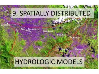
9. SPATIALLY DISTRIBUTED HYDROLOGIC MODELS
Single Cell in Landscape Evapo- transpiration Precipitation Atmosphere Land Surface Overland flow Sub-surface Sub-surface flow
Single Cell in Landscape But Outflow in Which Direction? Evapo- transpiration Precipitation Atmosphere Land Surface Overland flow Sub-surface Sub-surface flow
Flow Direction from DEM TIRIBIELEV all elevations in meters Which way out of cell H9?
Flow Direction from DEM TIRIBIELEV all elevations in meters Which way out of cell H9?
Flow Direction from DEM TIRIBIELEV all elevations in meters Which way out of cell I9?
Flow Direction from DEM TIRIBIELEV all elevations in meters Which way out of cell I9?
Flow Direction from DEM TIRIBIELEV all elevations in meters Which way out of cell I10?
Flow Direction from DEM TIRIBIELEV all elevations in meters Which way out of cell I10?
Computation of Travel Time How Fast? ~ Manning V = f(D, S, n) Slope: From DEM Manning’s n: From channel characteristics Depth: Field estimates Travel time? ~ Distance/V Distance: From flow net to river outlet (Electriona) Each cell can be assigned a travel time for water to reach the outlet.
“ “
Scenario 1: Rainfall falling uniformly spatially (but not temporally)
0.5 “ in first hour Contribution to flood hydrograph
2” in second hour Combined contributions to flood hydrograph.
1 “ in third hour Combined contributions to flood hydrograph.
Scenario 2: Rainfall falling variably over space, but uniformly over time) 1 2 3 Precipitation not only varies temporally, but also spatially. Can use simple technique like Thiessen polygons to alter inputs to various parts of basin.
Each polygonal area corresponds to a differing set of travel times or isochrones. Rain falling at same time in yellow area will reach outlet later than that in orange area. Rain falling in green area will all arrive at outlet within a 7 hour period, while the rain falling on the orange area will be distributed over a 19 hour period.
Time of Arrival of Cell/Polygon Contributions at Electriona.
SPATIAL VARIABILITY OF INPUTS • Assume that a storm occupies the entire Tiribí basin, but that the quantity of rain it delivers increases towards the headwaters. • As the air is forced to rise it produces greater precipitation at higher elevations. • The low lying orange area receives Excess precipitation of 0.5”.
Response of low lying area to excess precipitation of 0.5 “ in the first hour. Time distributed contribution of lowland areas’ excess precipitation at Electriona.
Response at Electriona to higher areas of the Jorco and Cañas receiving excess precipitation of 1.0” falling during the hour of the storm. Combined effects at Electriona of both the lower (faster, temporally dispersed response, but less excess precipitation), and upper (slower, less dispersed response, to large excess precipitation) parts of the basin.
Response at Electriona to highest areas of the Chiquito and Tres Ríos receiving excess precipitation of 2.0 mm falling during the hour of the storm, but requiring longer travel times to reach the outlet. Combined effects at Electriona of spatially varying excess precipitation inputs falling on cells with varying travel times to outlet. Basically becoming “wetter” as one proceeds away from the outlet.
Now Assume that Low Areas Receive Most Rain from the Storm and Upper Areas the Least
Arbitrarily set a discharge of 4 as a critical flood level • Flood Starts later. Storm Max in Highlands • Flood Starts earlier. Storm Max in Lowlands
Arbitrarily set a discharge of 4 as a critical flood level • Flood Starts later. • Peaks at same time. Storm Max in Highlands • Flood Starts earlier. • Peaks at same time. Storm Max in Lowlands
Arbitrarily set a discharge of 4 as a critical flood level • Flood Starts later. • Peaks at same time. • Lower peak above threshold. Storm Max in Highlands • Flood Starts earlier. • Peaks at same time. • Higher peak above threshold. Storm Max in Lowlands
Arbitrarily set a discharge of 4 as a critical flood level • Flood Starts later. • Peaks at same time. • Lower peak above threshold. • Fewer hours of inundation. Storm Max in Highlands • Flood Starts earlier. • Peaks at same time. • Higher peak above threshold. • More hours of inundation. Storm Max in Lowlands
Scenario 4: Rainfall falling variably over both time and space. 6. 5. 4. 3. 1. 2.