Macroscale hydrological modeling
Macroscale hydrological modeling. Dennis P. Lettenmaier Department of Civil and Environmental Engineering University of Washington IAI La Plata Basin Graduate Summer School Itaipu, Brazil November 10, 2009. Outline of this talk. Macroscale hydrological modeling strategy

Macroscale hydrological modeling
E N D
Presentation Transcript
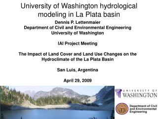
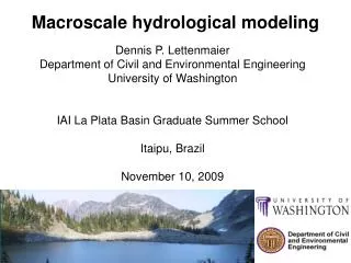
Macroscale hydrological modeling Dennis P. Lettenmaier Department of Civil and Environmental Engineering University of Washington IAI La Plata Basin Graduate Summer School Itaipu, Brazil November 10, 2009
Outline of this talk Macroscale hydrological modeling strategy Some aspects of model structure – the Variable Infiltration Capacity model as an example Model calibration Model evaluation and testing
Use of Models Applications Forcings Modeling • Precipitation • Temperature • Radiation • Vegetation • Atmospheric model output • Forecasting • Land Use change assessment • Climate change assessment • Wildfire Forecast Land Surface Hydrology Model (VIC)
Differences between macro-scale land surface hydrology models and traditional hydrology models
The Variable Infiltration Capacity (VIC) macroscale hydrology model
Development of the VIC Model Liang et al. (JGR, 1994 – standard reference for model) 2-layer soil vegetation model designed to be dynamically coupled to GCMs or weather models (e.g. at 5 degree lat lon resolution) Parameterized infiltration and base flow schemes Single layer energy balance snow model Physically-based vegetation model including canopy effects Physically-based evaporation based on the Penman/Monteith approach
Historic Use of the Model Despite the original conception of the model, until very recently the vast majority of the hydrologic research using the model has implemented the model in an “off-line” configuration. That is, driving data is produced (either from observations or simulations) and the model is run as a stand alone tool often as a “black box” used to interpret the hydrologic implications of the variations in the driving data. Most of the improvements in the model have come about because of the discovery of shortcomings of the model during the course of investigations focused on particular “off line” applications. In the last several years, as computational constraints have been relaxed somewhat and the importance of the land surface state as an important driver of atmospheric circulation and precipitation variability, more attention has been focused on using the tool in a dynamic setting. Precipitation and temperature bias remain difficult elements of fully coupled models to resolve. (I.e. it is often difficult to realize the benefits of an improved land surface scheme if precipitation or temperature in the coupled application are strongly biased for other reasons.)
Simulation Modes Water balance: Assumes that surface temperature = surface air temperature, hance ground het flux = 0, and once Lh is computed (given Rnet, surface wind, humidity, and vegetation properties), Ls is by difference (hence balance closes by construct) Energy balance: Iterates on surface temperature that closes the water balance (Ts is a term in emitted longwave, and latent and sensible heat). This formulation is more physically correct than water balance, however it does come at a much greater (typically order of magnitude) computational requirement. Reference: http://www.hydro.washington.edu/Lettenmaier/Models/VIC/Technical_Notes/ NOTES_model_modes.html
Land Surface Hydrology Model PNW GB CA CRB 12 km 1/8th Deg. 12 km 1/8th Deg. Modelo de Nieve
Water Balance Qb= Baseflow Qd= Runoff P= Precipitation E= Evapotranspiration E1= bare soil Ec =Canopy Et=Transpiration Wn=Soil Moisture Kn(W)=Hydraulic Conductivity Dn(W)=Diffusivity Zn=Soil Depth n= layer
Runoff (Qd) • i=Infiltration • im=Maximum Infiltration • bi=Shape parameter • A=Fraction of the area • As=fraction of the saturated area • W1=Soil Moisture in Layer 1 • io=specific point of I capacity
Baseflow(Qb) Ds=Fraction of Dm Dm=Maximum subsurface flow W2c=Maximum soil moisture content Ws=Fraction of W2c W2= Soil moisture in layer 2 W2- Soil moisture in layer 2 Saturated Insaturated
Three Parameter Non-linear Baseflow Relationship The modeler selects Dmax, Ds, Ws. (Wmax is determined by the soil parameters.) Ws and Ds determine the x and y positions of the linear threshold in the curve. Dmax determines the maximum base flow when the lower layer is fully saturated. Dmax = 100 Ds = 0.2 Ws = 0.8
Vegetation (Canopy surface), topography, snow, soil representations
Equal Area Elevation Bands The number of bands is determined by the elevation gradient and a specified interval used in pre-processing (e.g. 1500 m/ 500m in the example). Having determined the number of bands, the bands are forced to have equal area by ranking the pixels in a high resolution DEM and dividing them into groups within the cell boundaries with equal numbers of pixels. Temperature and precipitation are different in each band, but are keyed to the driving data for each cell. In current model implementations the mosaic of vegetation types is identical in each elevation band. High Elevation Band Medium Elevation Band Low Elevation Band
Representation of the Canopy and Canopy Storage Precipitation Canopy evap (wet canopy or snow) Transpiration (dry canopy) Canopy Storage (determined by LAI) Canopy “throughfall” occurs when additional precipitation exceeds the storage capacity of the canopy (rain or snow) in the current time step.
Vegetation Characteristics • The model represents a particular vegetation class primarily by: • Canopy albedo • Seasonal Leaf Area Index (LAI)– can be unique for each cell. • Canopy storage (assumed to be a function of LAI) • Characteristic vegetation roughness and displacement height • Stomatal resistance (evaporative resistance associated with transpiration) • Architectural resistance (evaporative resistance related to humidity gradient within the canopy structure as compared to the free air) • Rooting depth • Radiation attenuation factor (used to attenuate incoming solar radiation)
Evapotranspiration in VIC model wet canopy evaporation ET dry canopy transpiration bare soil surface evaporation
Evaporation and Transpiration Evaporation from wet vegetation and transpiration from dry vegetation are estimated by the physically-based Penman Monteith approach. The equation has the form: Evap = (Term1 + Term 2) / (Term 3) (see e.g. equation 3 in Wigmosta et al. 1994) Term 1 is net radiation term, which is primarily a function of incoming solar radiation (cloudiness) and the slope of the saturated vapor pressure-temperature curve. Term 2 is the vapor pressure deficit term which is primarily a function of the humidity and temperature of the air, scaled by an aerodynamic resistance term related primarily to wind speed and surface roughness. Term 3 is a function of the slope of the saturated vapor pressure and resistance terms associated with canopy resistance and aerodynamic resistance Bare soil calculations are similar but include a resistance term related to the soil’s ability to deliver moisture to the surface (a function of upper layer moisture content and soil characteristics)
Overall Modeling Structure for Evaporation Calculations Key drivers such as net radiation budget and wind speed are calculated explicitly for each component of the land surface (canopy, understory, bare soil, and snow surface). Wet or dry vegetation is incorporated by selecting the canopy resistance term (same equation). Overstory Understory Wet Vegetation Dry Vegetation Snow No Snow
Energy Balance Snow Model http://www.ce.washington.edu/pub/WRS/WRS161.pdf
Partitioning of Rain and Snow The model currently uses a very simple partitioning method to determine the initial form of the precipitation. E.g. RainMin= 0.0 C SnowMax = 2.0 C If T <= RainMin then 100% snow. If T >= SnowMax the 100% rain. Values in between are a linear interpolation between the two values. E.g. simulated precipitation at 0.5 degrees C would produce 75% snow, 25% rain.
Effects of Forest Canopy on Snow Accumulation Loss of canopy increases the snow water equivalent and increases the rate of melt. Source: Storck, P., 2000, Trees, Snow and Flooding: An Investigation of Forest Canopy Effects on Snow Accumulation and Melt at the Plot and Watershed Scales in the Pacific Northwest, Water Resources Series Technical Report No. 161, Dept of CEE, University of Washington. http://www.ce.washington.edu/pub/WRS/WRS161.pdf
Representation of Soil Column True depth and composition of the soil column is usually imperfectly known. Porosity, Ksat, field capacity, wilting threshold, residual capacity and other soil characteristics are determined from estimates of soil composition Storage capacity of each layer is depth times porosity. Rooting distribution is specified in the vegetation file as the fraction of the roots occurring in each depth range. The model then calculates the fraction of roots in each soil layer. Thus the rooting depths and soil layers can be varied independently. ~10cm Infiltration and surface runoff Interflow processes ~20cm Baseflow processes ~1.5 m
Model Combinatorial Algorithm Each cell is completely independent of the others. The model solves the water and energy balance independently for each elevation band and vegetation type within the cell (plus bare soil). Band 1 Band 2 . . . Band N Then in each time step the model creates a linear combination of each variable according to the fraction of the cell area that is associated with each band and veg type. Veg 1 . . Veg M Final Model Output Value Veg 1 . . Veg M Area fraction weighting by variable Veg 1 . . Veg M
Energy Balance Rn= Absorbed Radiation f(Ts,Albedo, Sw, Lw) H=Sensible Heat Flux f(rw,Ta, Ts, ra ,Cp) rwLeE=Latent Heat Flux f(ro, W,Ts) G=Ground Heat Flux f(Ts, T1, thermal conductivity, Z1) DHs=Change Energy Storage f(ra,Cp, Ts) Iteratively solved for Ts
Sub-daily air temperature (°C) Surface albedo (fraction) Atmospheric density (kg/m3) Precipitation (mm) Atmospheric pressure (kPa) Shortwave radiation (W/m2) Daily maximum temperature (°C) Daily minimum temperature (°C) Atmospheric vapor pressure (kPa) Wind speed (m/s) Model Forcing Data Below is an example of a 4 column daily forcing file: Pcp Tmax Tmin Wind 6.000 22.560 6.440 3.320 1.775 20.800 4.480 1.260 0.000 25.870 4.360 0.970 0.000 28.470 4.610 1.400 0.000 26.130 8.680 0.880 0.500 25.280 6.860 1.770 ...
Forcing Data Preprocessor The driving data for the model can be explicitly given as a time series, or the model will construct a set of complete forcings from a set of limited daily observations (usually daily precip, tmax, tmin, wind speed) following methods developed by Thornton and Running (1997). Hourly temperature data (needed for the hourly snow model simulations) are reconstructed based on empirical relationships to Tmax and Tmin. Cloudiness and solar radiation attenuation and incoming long wave radiation are estimated via the diurnal temperature range. Dew point temperature is related to daily minimum temperature with a long wave radiation correction.
2604 60km×60km grid cell 黄河流域 淮河流域 长江流域
Result: Daily Precipitation, Tmax, Tmin 1915-2003
Overview of Data Processing Steps • Collect observed station data and preprocess wind data • Reformat station data to an irregularly spaced gridded file. • Regrid the raw station information to the VIC lat lon grid. • Quality control to remove implausible values • Adjust gridded raw station data to remove station inhomogeneities using HCN or HCDN data sets as a standard (optional) • Topographic adjustment of precipitation data (using PRISM data as a standard). • Reformatting to final file format needed by VIC.
Regridding Details Symap regridding algorithm accounts for station proximity via an inverse square weighting, but also accounts for the independence of the stations from one another. The interpolation scheme ensures that collectively these two nearly coincident stations are assigned about the same weight as each of the other two stations.
Hydro1k (all continents) http://edc.usgs.gov/products/elevation/gtopo30/hydro/index.html
Digital Elevation Models Hydro1k: equal area projection, 1 km res. Gtopo30 or SRTM30: geographic projection, 30 arc-seconds http://edc.usgs.gov/products/elevation/gtopo30/gtopo30.html http://topex.ucsd.edu/WWW_html/srtm30_plus.html
Land Cover Classification U. Maryland AVHRR, 1 km global product http://glcf.umiacs.umd.edu/data/landcover/ IGBP, 3 arc-minute global product http://landcover.usgs.gov/globallandcover.php
Soil Information • UNESCO/FAO global soil maps • http://www.lib.berkeley.edu/EART/fao.html
Example: Basin Delineation
Method 1: • Use Hydro1k Basin Delineations • Best for larger basins • faster process • Method 2: • Use ArcInfo Functions to Delineate a Basin • Any size basin – all small watersheds • Uses a high-resolution DEM to delineate
Why process VIC output? What we typically want: Hydrograph at various points in stream network Monthly average water and/or energy budget of a basin What VIC (currently) gives us: Moisture and energy fluxes and states for individual grid cells Output interval = model time step We generally must process VIC’s output before we can use it
VIC assumptions & routing Most other models run in “image” mode For each time step, they compute fluxes and state for all grid cells VIC currently runs in “vector” mode For each grid cell, it runs the entire simulation period (all time steps) This means each grid cell’s water and energy balance is independent of its neighbors
Why can VIC get away with this behavior? Assumptions: The vast majority of grid cell runoff goes into the grid cell’s local channel network Very little runoff goes from one grid cell’s soil to its neighbor’s soil Water from the channel does not recharge into the soil (water transport is one-way)
Why can VIC get away with this behavior? These assumptions are valid if: Grid cells are large (typically we have 1/8 degree; 12.5 km on a side) Groundwater flow is small relative to surface and near-surface flow Lakes/wetlands do not have significant channel inflows Flooding (over banks) is insignificant These conditions hold most of the time
Consequences VIC gives us a separate set of output files for each grid cell VIC does not (currently) perform channel routing of runoff VIC does not give us a hydrograph Routing is performed by a stand-alone program (“rout”) A benefit: VIC uses very little memory system only needs to store state and fluxes of one grid cell at a time
How to get a hydrograph Routing program: “rout” Takes VIC fluxes files for all cells in basin Reads daily runoff and baseflow totals Convolves local (runoff+baseflow) with unit hydrograph response function Adds local hydrograph response to flow from upstream Propagates flow downstream Runoff + baseflow Runoff + baseflow Runoff + baseflow Runoff + baseflow
3. Model calibration (“the Achilles heel of hydrological modeling”)