Download
1 / 33
330 likes | 507 Vues
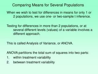
Comparing Means for Several Populations. When we wish to test for differences in means for only 1 or 2 populations, we use one- or two-sample t inference. Testing for differences in more than 2 populations, or at several different levels (values) of a variable involves a different approach.

E N D
Comparing Means for Several Populations When we wish to test for differences in means for only 1 or 2 populations, we use one- or two-sample t inference. Testing for differences in more than 2 populations, or at several different levels (values) of a variable involves a different approach. This is called Analysis of Variance, or ANOVA. ANOVA partitions the total sum of squares into two parts: within treatment variability between treatment variability
Comparing Means for Several Populations Example: Test 5 types of concrete for differences in moisture absorption. The 5 types of concrete are the five levels of the treatment. Within Variability – this seeks to quantify the variability in absorption for one particular type of concrete. Between Variability – this seeks to quantify the differences between the types of concrete. ANOVA seeks to answer the question “Are the differences between the 5 sample means what is expected purely from random variation alone?”
Definitions • An experimental unit is an object, or subject, that produces a sample measurement. • The experimental conditions that define the different populations in a completely randomized design are called treatments. • Testing for differences in the treatments is equivalent to testing for differences inthe population means.
Practice on Definitions • See page 399 section 10.1 exercises.
Graphical demonstration: Employing two types of variability
30 25 20 19 12 10 9 7 1 Treatment 3 Treatment 1 Treatment 2 20 Graphical demonstration: Employing two types of variability 16 15 14 11 10 9 A small variability within the samples makes it easier to draw a conclusion about the population means. The sample means are the same as before, but the larger within-sample variability makes it harder to draw a conclusion about the population means. Treatment 1 Treatment 2 Treatment 3
Assumptions for ANOVA • 1. The samples are independent • Selection of objects from any one population is unrelated to the selection of objects from any of the other populations. Selections are random. • Examples • Different groups of people (no person in more than one group) • Different types of music • Different concentrations of chemicals • Different models of automobiles
Assumptions for ANOVA • 2. Each population has the same standard deviation, s. But the values of the population standard deviations is not known before testing.
Assumptions for ANOVA • 3. Each sample has a mean that can be calculated. This mean is somehow representative of the population mean for its population.
Assumptions for ANOVA • 4. Each population is normally distributed • Quantitative data: sample size is at least 30 • However, we will assume normally distributed populations for all the problems we work.
Assumptions for ANOVA The following assumptions are required for a 1-way ANOVA: The k populations are independent. Each population has common standard deviation, s. Each population has a mean, mi for i = 1, 2, …, k. Each population is normally distributed. So we now are testing whether all the treatment means are equal. H0: m1 = m2 = … = mk Ha: At least two of the population means are not equal
Test Statistic • If the null hypothesis is true, we expect the k sample means to have reasonably similar values. • In other words, if the population means are equal, we would expect the variability among the sample means to be relatively small. • Variability among the sample means is one of the things we will be testing for.
Test Statistic • If the null hypothesis is true, we do not expect the population means to be exactly the same, because there is a chance factor in our choice of sample experimental units. • We need to take into account the variability due to chance among the sample means.
Test Statistic • This method is called “analysis of variance” of ANOVA because we are comparing two sources of variance: the variance among the sample means and the variation expected by chance among the sample means when the null hypothesis is true.
Test Statistic • Our test statistic is called F. • F = Variability among the sample means Variability expected by chance
Degrees of freedom • For a sample, (or group) (k) df = n – 1 • Total df = total number of units in the experiment – 1 • Error df = Total df – Group df • Or • Error df = N - k
Minitab • We will use Minitab to do our calculations. • A typical Minitab display is on the next slide.
ANOVA Table: Tensile Strength for 6 Machines Analysis of Variance for Tensile-Strength Source DF SS MS F P Machine 5 5.34 1.07 0.31 0.902 Error 18 62.64 3.48 Total 23 67.98 SSMachine = 5.34 (sample mean variability), k = 6 machines SSError = 62.64 (variability due to chance) Notice how much larger the “chance” variability is than the other. There is little to no evidence that the machines differ in mean tensile-strength. Look at that HUGE p-value!
Another Minitab Example • Example 102 page 369 • Sociologist and GPA college students
One-way ANOVA: GPA versus Group Source DF SS MS F P Group 3 1.519 0.506 2.99 0.044 Error 36 6.091 0.169 Total 39 7.610 S = 0.4113 R-Sq = 19.96% R-Sq(adj) = 13.29% Individual 95% CIs For Mean Based on Pooled StDev Level N Mean StDev ---+---------+---------+---------+------ Lower Middle 10 2.5240 0.4362 (--------*--------) Poor 10 2.2640 0.3161 (-------*--------) Upper Middle 10 2.7170 0.4125 (--------*-------) Well-to-do 10 2.7560 0.4653 (--------*--------) ---+---------+---------+---------+------ 2.10 2.40 2.70 3.00 Pooled StDev = 0.4113
Manual Calculation • The formula for calculating F using the Mean Square Treatment is given on page 375.
Manual Calculation • To determine the p value when the f value is known, we need to use a table. • Table 5 is on pages VII, VIII, IX in the table appendix. • In general, Table 5 will provide only approximate p-values. To find precise values, technology is needed.
ANOVA – What is expected from you? Be able to complete each of the following exercises: State the two hypotheses. What is the observed value of the test statistic? (F = ?) Is this valid? We will typically “assume” the method is ok. What is the p-value? State a conclusion. Using a table for comparisons, locate what mean(s) are significantly different if you accepted the alternative hypothesis. (Sect 10.3)
Analysis of Variance results:Responses stored in Score. Factors stored in Hair Color. Factor means ANOVA table
Example Page 423 # 1 One-way ANOVA: Score versus Hair Color Source DF SS MS F P Hair Color 3 908.8 302.9 5.44 0.007 Error 20 1113.0 55.7 Total 23 2021.8 H0: mlight_blond = mdark_blond = … = mdark_brunette Ha: At least two population means are different. Accept Ha if p-value < 0.05 F = 5.44 p-value = 0.007 At the 0.05 level of significance, there is sufficient evidence to conclude that there is a difference among mean pain thresholds for people possessing these four hair colors.
10.3 Which means are different?Multiple Comparisons • When an analysis of variance F-test indicates a significant difference among population means, (accept Ha), the next question is which means are different.
Which means are different? • We need to test each of the following pairs of hypotheses. • Pair 1: Ho: μ1-μ2=0 Ha: μ1-μ2≠0 • Pair 2: Ho: μ1-μ3=0 Ha: μ1-μ3≠0 • Pair 3: Ho: μ2-μ3=0 Ha: μ2-μ3≠0
Which means are different? • To test each pair of hypothesis, we are only testing two means for a difference between them. • This is the two-sample t-statistic that we used in section 9-2. • However, we will substitute MSE(Mean Square Error) for s2 • See page 416 for entire equation.
Which mean is different? • We can use StatCrunch to calculate the value of t and the p-value for each of the comparisons. We can then draw our conclusions based on the p-value for each pair (is it less than α? If so we accept the alternative hypothesis), and summarize our findings in a chart. This is how the revised section in the book does it. • See example 10.4 p 418
Multiple Comparisons Let’s look further at the example on hair coloring
Summary • Ex 10.5 summarizes ideas from Chapter 10. See p 421
When should we use the multiple comparison method? • The sample data are obtained from the k populations using a completely randomized design • An analysis of variance F-test indicates that there are some differences among the k population means. • The objective is to determine which of the k population means differ. It is usually of interest to determine which mean might be the largest (or smallest).