Download
1 / 39
390 likes | 518 Vues
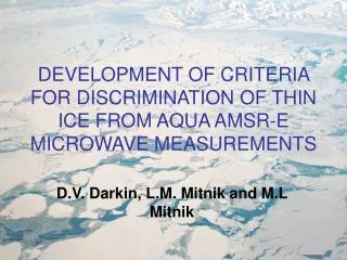
DEVELOPMENT OF CRITERIA FOR DISCRIMINATION OF THIN ICE FROM AQUA AMSR-E MICROWAVE MEASUREMENTS. D.V. Darkin, L.M. Mitnik and M.L Mitnik. Study of thin ice in marginal seas of Asia. Subject: Sea ice, namely thin ice Location: Sea of Okhotsk and Sea of Japan Satellite: Primarily Aqua;

E N D
DEVELOPMENT OF CRITERIA FOR DISCRIMINATION OF THIN ICE FROM AQUA AMSR-E MICROWAVE MEASUREMENTS D.V. Darkin, L.M. Mitnik and M.L Mitnik
Study of thin ice in marginal seas of Asia • Subject: • Sea ice, namely thin ice • Location: • Sea of Okhotsk and Sea of Japan • Satellite: • Primarily Aqua; • Sensors: • Passive microwave radiometer, AMSR-E; • Spectoradiometer, MODIS;
Motivation • We have found that modern concentration algorithms have problems with thin ice formed in coastal polynias in the Okhotsk and Japan seas; • Basic Bootstrap and NASA Team 2 Algorithms as provided in data granules from NSIDC[1]; • Ice concentration of consolidated thin ice types (dark nilas < 5 cm, light nilas >5 <10 cm) is underestimated roughly by 20%-40%; • Paper submitted, peer reviewed, being corrected [2];
Ice concentration Looks roughly About 60% NT2 Ice concentration of Okhotsk Sea. 14 February 2003, Ascending Swath (Daytime)
Not so. How about near 100% ? NT2 Ice concentration of Okhotsk Sea. 14 February 2003, Ascending Swath (Daytime)
Examples • BBA IC • Aqua AMSR-E
NT2 IC • Aqua AMSR-E
MODIS reflectance field • Histogram equalized • 40-80% concentration • Boundaries from • BBA & NT2 on • MODIS (645 nM band reflectance)
Simple threshold classification • Used albedo values as references for thresholds;
NT2 BBA Same true for Tartar strait, Japan sea. 14 February 2003, Ascending Swath (3:35 GMT)
Left(MODIS Ch1)Right (rough classification of ice types, based on MODIS)
Experimental vs. modeled data • Using this approach and 12 cloud free days of collocated AMSR-E and MODIS Aqua data, 628 microwave pixels selected; • Brightness temperatures (Tb) spectra for 18.7 to 89 GHz Aqua channels Vertical and Horizontal polarizations were compared to spectra modeled using Radiative Transfer Modeling (RTM) [3]. • Significant differences in means were identified.
New emissivity coefficients derived • RTM helped derive approximations for estimating emissivity of thin ice;
Model dataset • RTM using [2]; • Uses emissivity for thin ice and for thicker ice types (grey ice, grey-white ice); • Accurate atmospheric influence modeled using meteorological data for typical Okhotsk sea winter conditions (ship and ground st. data); • Over 1600 points for thin ice of various concentrations; • Over 6500 point for first year ice of various concentrations; • Normally distributed noise added to various parameters to account for sensor noise and natural variability of atmospheric and oceanic parameters.
Dataset statistical properties SSW IC Standard Q <0.05 kg/m2 = 58% Sev atm Q > 0.05 kg/m2 =42% Standard W<10 kg/m2 = 89% Sev atm: W > 10 kg/m2 =11% w Q
What’s next? • We have 8x8000 array of accurately modelled Tb for 4 ASMR-E frequencies (18.7, 23.8, 36.5, 89 GHz), and two polarizations V.,H.-Pol; • Dimensionality reduction (Feature extraction). Possibly non-linear. Need to construct 2-3 dimensional feature space; • Create a discriminant function separating this space in two halves each containing thin ice and thick ice as points;
Experiment • Full search is computationally possible for 2-D or 3-D feature spaces; • Use simpler linear methods for creation of discriminant function, but use large feature-combination space [4]; • Robust linear regression selected for discriminant development;
Construction of discriminant function • For 2 features we need to find the best F1 and F2 such that Y = +1 for thin ice and Y=-1 for older ice, where 0 = decision boundary and A0 ,A1 ,A2 determined by regression; • Y = A0+ A1·F1+ A2·F2 • For 3 features we need to find the best F1 and F2 F3 such that Y = 1 for thin ice and Y=-1 for older ice, where 0 = decision boundary and A0 ,A1 ,A2 ,A3 determined by regression; • Y = A0+ A1·F1+ A2·F2 + A3·F3
Definition of features Fi, i=1,2,3 • Combine any 2 AMSR-E channels out of 8. • 7 types of combinations possible for the selected channels: • addition, subtraction, division, multiplication, normalized difference, log of sum, log of difference; • Normalized difference defined as f(a,b)=(a-b)/(a+b)
Perform full search • Best features are the one that lead to minimum number of misclassifications; • Brute force search was done without constraints, logging best results as they are found; • For 2 features the search space included over 200000 combinations including repetitions and took around several hours on a PC; • For 3 features the search included almost 90.000.000 combinations and took less than 24 hours.
Results for 2 features • For 2 features the best combination lead to 96.44% correct classifications on the model array; • F1=F(18.7V, 36.5H) = log(Tb(18.7V) + Tb(36.5H)) • F2=F(18.7H, 36.5H) = log(Tb(18.7H) + Tb(36.5H)) • Discrimination criteria based on these features was named C2 = A0+ A1·F1+ A2·F2
Results for 3 features • For 3 features the best combination lead to 97.11% correct classifications on the model array; • F1=F(18.7V, 89V) = (Tb (18.7V)-Tb (89V))/Tb (18.7V)+Tb (89V) • F2=F(24.8V, 89H) = log(Tb(24.8V) + Tb(89V) ) • F3=F(18.7H) = log(Tb(18.7H) ) • Discrimination criteria based on these features was named C3 = A0+ A1·F1+ A2·F2 + A3·F3
Limitations of the model • The model used in RTM process does not account for scattering in deep snow and cloud ice crystals; • Empirical filtering scheme was developed by utilizing relation Tb(36.5V) / Tb(89V) • If the relation exceeds 1.175 then we have scattering; • If we have scattering, then it’s not thin ice.
Back to NW Okhotsk sea and Tartar strait shown in the beginning C2 and C3 should show thin ice. Shouldn’t they?
Mean value of C2 criteria vs. MODIS reflectance Threshold = 0.75
Mean value of C3 criteria vs. MODIS reflectance Threshold = 1.0
Application of the criteria • C2 or/and C3 can be used to create a conditional probability density function P =P(C|Tbs) where C is the new ice, and Tb is vector of Tb. • Then for each pixel sensed by AMSR-E we can approximate IC as mixture of two ice concentrations : • IC = P ·ICthin + (1-P)·ICthick • Where ICthickcould be BBA, NT or any other IC algorithm and ICthin is determined with a special thin ice algorithm, that can be developed separately for thin ice modeled values;
Outlook • Validation using MODISALB, Albedo product for snow and ice announced on the web by NASA, but not available. Anyone heard anything? • Testing under variable conditions (spring melt, severe atmosphere contamination) • Other seas with highly productive polynyas; • Development of algorithm suite able to provide ice concentration and ice type information using the criteria
References • 1. D.V. Darkin, L.M. Mitnik and M.L Mitnik. Spectra of microwave emissivity of thin ice derived from Aqua measurements over the Japan and Okhotsk seas // Issledovanie Zemli iz Kosmosa (in Russian, submitted, 2007). • 3. http://www.nsidc.org/ • 2. Mitnik L.M., Mitnik M.L. Retrieval of atmospheric and ocean surface parameters from ADEOS-II AMSR data: comparison of errors of global and regional algorithms // Radio Sciences. 2003. V. 38, No. 4, 8065, doi: 10.1029/2002RS002659. • 4. Bishop C.M. Neural networks for pattern recognition.1995. Oxford University Press.