Download

1 / 51
520 likes | 649 Vues
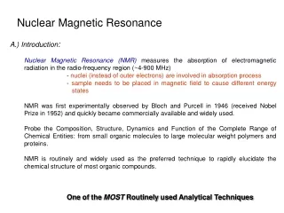
Join our Solid-State Nuclear Magnetic Resonance workshop led by Dieter Freude from the Institute für Experimentelle Physik I at the University of Leipzig. The workshop, held on May 21, 2008, at the Biotechnology Research Institute, Universiti Malaysia Sabah, covers key topics in NMR, including the principles of nuclear spin, gyromagnetic ratios, Zeeman splitting, and Larmor frequency. Gain insights into historic experiments and modern applications, including chemical shifts and the significance of shielding effects in NMR spectroscopy.

E N D
Solid-state nuclear magnetic resonance.Workshop • Dieter Freude, Institut für Experimentelle Physik I der Universität Leipzig Lecture in the Biotechnology Research Institute, Universiti Malaysia Sabah, 21 May 2008
Harry Pfeifer's NMR-Experiment 1951 in Leipzig H. Pfeifer: About the pendulum feedback receiver and the obsevation of nuclear magnetic resonances, diploma thesis, Universität Leipzig, 1952
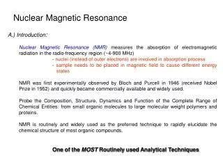
How works NMR: a nuclear spin I = 1/2 in an magnetic field B0 Many atomic nuclei have a spin, characterized by the nuclear spin quantum number I. The absolute value of the spin angular momentum is The component in the direction of an applied field is Lz = Iz m = ½ for I = 1/2. Atomic nuclei carry an electric charge. In nuclei with a spin, the rotation creates a circular current which produces a magnetic moment µ. An external homogenous magnetic field B results in a torque T = µ Bwith a related energy of E = -µ·B. The gyromagnetic (actually magnetogyric) ratio g is defined by µ = gL. The z component of the nuclear magnetic moment is µz = gLz = g Izg m . The energy for I = 1/2 is split into 2 Zeeman levels Em = -µz B0 = -g mB0 = gB0/2 = wL/2. Pieter Zeeman observed in 1896 the splitting of optical spectral lines in the field of an electromagnet.
Larmor frequency Classical model: the torqueT acting on a magnetic dipole is defined as the time derivative of the angular momentum L. We get By setting this equal to T = µ B , we see that The summation of all nuclear dipoles in the unit volume gives us the magnetization. For a magnetization that has not aligned itself parallel to the external magnetic field, it is necessary to solve the following equation of motion: We define B =(0, 0, B0) and chooseM(t= 0) = |M| (sina, 0, cosa). Then we obtain Mx= |M| sina coswLt, My= |M| sina sinwLt, Mz= |M| cosa with wL =-gB0. The rotation vector is thus opposed to B0for positive values of g. The Larmor frequency is most commonly given as an equation of magnitudes: wL =gB0 or Joseph Larmor described in 1897 the precession of electron orbital magnetization in an external magnetic field.
Some of the 130 NMR isotopes R. K. Harris, E. D. Becker, S. M. C. de Menezes, R. Goodfellow, P. Granger:NMR nomenclature: Nuclear spin properties and conventions for chemical shifts - IUPAC recommendations 2001, Pure Appl. Chem. 73 (2001) 1795-1818
shielded magnetic field B0(1-s) external magnetic field B0 OH- H+ electron shell Chemical shift of the NMR We fragment hypothetically a water molecule into hydrogen cation plus hydroxyl anion. Now the 1H in the cation has no electron shell, but the 1H in the hydroxyl anion is shielded (against the external magnetic field) by the electron shell. Two signals with a distance of about 35 ppm appear in the (hypothetical) 1H NMR spectrum.
1, 2HTMS 6, 7Li1M LiCl 11B BF3O(C2H5)2 13CMS = (CH3)4Si 14, 15NNH4+ 19FCFCl3 23Na1M NaCl 27Al[Al(H2O)6]3+ 29Si TMS = (CH3)4Si 31P85% H3PO4 51V VOCl3 129, 131XeXeOF4 1000 100 10 0 -10 -100 -1000 d/ ppm Chemical shift rangeof some nuclei An NMR spectrum is not shown as a function of the frequency n = (g / 2p) B0(1-s), but rather on a ppm-scale of the chemical shift d= 106(nref-n) /nL, where the reference sample is defined by UPAC, e. g. TMS (tetramethylsilane) for 1H, 2H, 13C, and 29Si NMR. Ranges of the chemical shifts of a few nucleiand the reference substances, relative to which shifts are related.
Offset The basic frequency is 400.13 MHz for 1H (AVANCE 400). For other nuclei, the value with 6 characters after the decimal point is given in tables. Having a correct adjusting of the external magnetic field and no offset,the transmitter frequency equals the basic frequency, and we obtain the position of 0 ppm exact in the middle of the spectral range. An offset can be obtained by using the commands O1 in channel F1 or O2 in Channel F2 and setting the values 0 Hz. Then the transmitter (carrier) frequency equals the sum of basic frequency and offset, e.g. in channel F1 we have SFO1 = BF1 + O1. But we obtain the position of the offset frequency exact in the middle of the spectral range, since the referencing of the scale in Hz or ppm is performed with respect to the basic frequency. With other words, changing the offset does not change the ppm-value of an NMR signal. Note that the transmitter frequency offset is not identical with the signal offset. However, the ppm-value of an NMR signal can be changed by using the command SR. For solid-state NMR the use of SR is not recommended. Set always SR = 0 and reset SR = 0 after changing the nucleus (special feature of xWinNMR), but check the value "Field" on the hardware panel.
Shimming and adjusting the magnetic field with PDMS Polydimethylsiloxane (PDMS, [-Si(CH3)2-O-]n) has a chemical shift of 0.07 ppm. It should be run at nrot = 35 kHz. Keep the sample permanent in a rotor. Shimming and field adjusting must be performed for each probe. It should be done again, if the probe has been repaired or a stupid person changed the data. Always read the proper shim file for the probe and check the value "Field". MAS shimming is much more simple than shimming a liquid-state spectrometer. For shimming and adjusting use the gs command (go setup) and call bsmsdisp.Shimming target is either a very long mono-exponential decay of the free induction or a maximum Lorenz-shaped signal in the frequency domain (frq).Bruker MAS probes have usually the rotor in the y-z-plane. Thus x = 0.Shim first z and y alternating, if necessary then x2-y2 and xy. Keep 0 for other. Lorenz-shape is often not achieved. A 50% narrow signal about 10 Hz broad plus a 50% signal 40 Hz broad are sufficient. Only after shimming (or reading the shim file) the "Field"-value has to be adjusted (or checked). Use an offset of 0.07 ppm (28 Hz for AVANCE 400). Change "Field" until the signal is in resonance. "Field" amounts 7200 with 4.shim at 25 April 2008. 87 Field units correspond to 400 Hz 1H-shift or to 1 ppm for all nuclei.
Fourier transform NMR History Continuous wave (cw) spectrometers with stationary rf input (omit dotted box) are rarely applied these days. To prevent saturation, cw spectrometers use a weak rf input of a few µT at constant frequency with variable magnetic field or vice-versa. Pulse spectrometers use radio frequency pulses. In the study of liquids, rf induction in the mT range is sufficient, whereas in the study of solids, maximal rf induction and minimal pulse width is desired, for example: 12 mT with an pulse lengthtp/2 of 1 µs is necessary to rotate the magnetization of 1H-nuclei from the z-direction into the x-y-plane.
Free induction and Fourier transform The figure shows at left thefree induction decay (FID)as a function of time and at right the Fourier transformed 1H NMR spectrum of alcohol in fully deuterated water. The individual spikes above are expanded by a factor of 10. The singlet comes from the OH groups, which exchange with the hydrogen nuclei of the solvent and therefore show no splitting. The quartet is caused by the CH2 groups, and the triplet corresponds to the CH3 group of the ethanol. The splitting is caused by J-coupling between 1H nuclei of neighborhood groups via electrons.
Jean Baptiste Joseph Fourier’s transformation Fourier’s original form from 1822 was conceived to describe the spatial distribution of temperature by infinite sums. In spectroscopy, it is mainly used to transform signals from the time domain into the frequency domain and vice-versa. The symmetric form of the Fourier transform is written Note that exp(iw0t) = cosw0t + i sinw0t. Let us now consider the function g(t) = exp(-t / Td + iw0t). The Fourier transform is Setting w0 = 0, we see that the Fourier transform of a mono-exponential decay gives f(w) = 1 / (1 + w2Td2). In this case there is no imaginary part of the frequency domain. But usually we have real part und imaginary part in the time and frequency domain as well.
Lorentz line shape A mono-exponential decay of the free induction corresponds to G(t) = exp(-t/T2), where T2 denotes the transverse relaxation time. The Fourier-transform gives fLorentz = const. 1 / (1 + x2) with x = (w-w0)T2, see red line. The "full width at half maximum" (fwhm) in frequency units is
Advantage of FT NMR compared to cw NMR Supposed, we would measure the signal in the frequency domain by cw NMR. Then we would measure a signal only in the narrow intervals. The time we spend for measuring the broad intervals is lost. But for very broad signals, with other words for a very short FID, the dead time of the pulse spectrometer causes a disadvantage compared to the cw technique.
Sampling theorem The sampling theory named after Harry Nyquist tells us that for the unique identification of a cosine function, at least two measurements must be taken per oscillation period. For the duration of the sampling of a measurement value (dwell time) t we then get t < 1/(2n) or in other words, the sampling rate has to be at least twice the oscillation frequency to be measured. If the sampling rate is exactly double or less, we get, after Fourier transformation, mirror symmetric replicates or aliasing. These are mirrored into the unique spectral range from 1/(2t) from outside. If the sampling rate is much higher than twice the frequency of the sampled signal, no advantage is gained in non-noisy signals. This so-called oversampling, however, simplifies the determination of signals buried in noise. The figure shows measurements with a dwell time of 1 ms. Thedashed line with a frequency of 250 Hz has 4 measured values per period (double oversampling). The dotted 500 Hz line contains only 2 measured values per period and, after a Fourier transformation, would appear on both edges of the frequency range from 0 to 500 Hz, since it is indiscernible from 0 Hz (all points pass through a line).The straight line for 0 Hzyields the same result. The 1 kHz line contains only one measured point per period and would be mirrored in to both edges of the measurement range.
Sampling theorem The sampling theory named after Harry Nyquist tells us that for the unique identification of a cosine function, at least two measurements must be taken per oscillation period. For the duration of the sampling of a measurement value (dwell time) t we then get t < 1/(2n) or in other words, the sampling rate has to be at least twice the oscillation frequency to be measured. If the sampling rate is exactly double or less, we get, after Fourier transformation, mirror symmetric replicates or aliasing. These are mirrored into the unique spectral range from 1/(2t) from outside. If the sampling rate is much higher than twice the frequency of the sampled signal, no advantage is gained in non-noisy signals. This so-called oversampling, however, simplifies the determination of signals buried in noise. The figure shows measurements with a dwell time of 1 ms. Thedashed line with a frequency of 250 Hz has 4 measured values per period (double oversampling). The dotted 500 Hz line contains only 2 measured values per period and, after a Fourier transformation, would appear on both edges of the frequency range from 0 to 500 Hz, since it is indiscernible from 0 Hz (all points pass through a line).The straight line for 0 Hzyields the same result. The 1 kHz line contains only one measured point per period and would be mirrored in to both edges of the measurement range.
Sampling theorem The sampling theory named after Harry Nyquist tells us that for the unique identification of a cosine function, at least two measurements must be taken per oscillation period. For the duration of the sampling of a measurement value (dwell time) t we then get t < 1/(2n) or in other words, the sampling rate has to be at least twice the oscillation frequency to be measured. If the sampling rate is exactly double or less, we get, after Fourier transformation, mirror symmetric replicates or aliasing. These are mirrored into the unique spectral range from 1/(2t) from outside. If the sampling rate is much higher than twice the frequency of the sampled signal, no advantage is gained in non-noisy signals. This so-called oversampling, however, simplifies the determination of signals buried in noise. The figure shows measurements with a dwell time of 1 ms. Thedashed line with a frequency of 250 Hz has 4 measured values per period (double oversampling). The dotted 500 Hz line contains only 2 measured values per period and, after a Fourier transformation, would appear on both edges of the frequency range from 0 to 500 Hz, since it is indiscernible from 0 Hz (all points pass through a line).The straight line for 0 Hzyields the same result. The 1 kHz line contains only one measured point per period and would be mirrored in to both edges of the measurement range.
Sampling theorem The sampling theory named after Harry Nyquist tells us that for the unique identification of a cosine function, at least two measurements must be taken per oscillation period. For the duration of the sampling of a measurement value (dwell time) t we then get t < 1/(2n) or in other words, the sampling rate has to be at least twice the oscillation frequency to be measured. If the sampling rate is exactly double or less, we get, after Fourier transformation, mirror symmetric replicates or aliasing. These are mirrored into the unique spectral range from 1/(2t) from outside. If the sampling rate is much higher than twice the frequency of the sampled signal, no advantage is gained in non-noisy signals. This so-called oversampling, however, simplifies the determination of signals buried in noise. The figure shows measurements with a dwell time of 1 ms. Thedashed line with a frequency of 250 Hz has 4 measured values per period (double oversampling). The dotted 500 Hz line contains only 2 measured values per period and, after a Fourier transformation, would appear on both edges of the frequency range from 0 to 500 Hz, since it is indiscernible from 0 Hz (all points pass through a line).The straight line for 0 Hzyields the same result. The 1 kHz line contains only one measured point per period and would be mirrored in to both edges of the measurement range.
Fast Fourier transform The numerical calculation is based on a a certain number of measured points, e. g. 1024 points, if size (SI) and time domain (TD) were set to 1K. The Integral (that means summation) has to be performed over the same number of points. Therefore, the calculation effort is increasing with the square of the size. Fast Fourier Transform (FFT) is a calculation procedure that reduces the effort in such a way that it is only proportional to the size. We have always for digital Fourier transforma dwell time (DW) of Dtand a correspondent sweep width (SWH) Dn = 1 / 2Dt or SWH = 1 / 2DW. Starting from the sweep width in ppm (SW = SWH/ SFO1, the latter given in MHz), the dwell time is calculated corresponding to this relation. In opposite to the analog acquisition mode, an oversampling is used for the digital acquisition mode. The size (SI) of the spectrum determines the number of points in the frequency domain. We have SI / 2 points in the real part and the same number in the imaginary part of the spectrum. Therefore, the frequency resolution (d denotes the distance between two points on the scale) equals dn = Dn / ½ SI = DW-1 / SI = SWH / SI or dppm = SW / SI. The time domain (TD) can be much shorter than SI.
Uref Basics for synthesis and detection of frequencies Addition theorem Operational amplifier + RC unit A phase sensitive detector (also known as a lock-in amplifier) is a type of amplifier that can extract a signal with a known carrier wave from noisy environment. It multiplies the signal voltage with an reference voltage coming from the same origin (look-in).
Quadrature detection After the preamplifier the same signal goes to two independent phase sensitive detectors having reference signals with the same frequency but a 90° shifted phase. Their output is the input of (two units of) the analogue-to-digital conversion (ADC). The ADC's create digital values each time interval of the dwell time DW. One value goes to the real part of the time domain, the next to the imaginary part and so on. It means that we have time intervals of 2DW between the measuring values in one part. The Fourier transform needs always real part and imaginary part of the spectrum. In addition it is based on the proper adjustment for analogue acquisition. It means the amplification of the both branches should be identical and the phase difference of the two references should amount exactly 90°. Otherwise we obtain a sharp peak exact in the middle of the sweep range and mirror signals with respect to the middle. No problems for fully digitalized acquisition.
The difference between solid-state and liquid NMR,e. g. the lineshape of water solid water (ice) Dn / kHz -10 -40 -30 -20 0 10 20 30 40 liquid water Dn / Hz -0.1 -0.4 -0.3 -0.2 0 0.1 0.2 0.3 0.4
H H Campher H Structure determination by NMR H C Structure NMR-Spektrum 1H-NMR 13C-NMR HH-COSY HC-COSY HETCOR NOESY R. Meusinger, A. M. Chippendale, S. A. Fairhurst, in “Ullmann’s Encyclopedia of Industrial Chemistry”, 6th ed., Wiley-VCH, 2001
Line broadening effects in solid-state NMR chemical shift anisotropy distribution of the isotropic value of the chemical shift dipolar interactions first-order quadrupole interactions second-order quadrupole interaction inhomogeneities of the magnetic susceptibility
Chemical shift anisotropy anisotropy asymmetry factor h = 0 h 0 Dwcsa
Distribution of isotropic values of the chemical shift No common model exists for this very important broadening effect.
1 = I 2 a = 2D w DDWW w 0 Dipolar broadening of a two-spin system = II,IS (3 cos2q - 1)
static MAS h = 0 h = 0.5 h = 1 16 16 32 4 5 14 - - - - - 1 0 0 9 9 9 21 6 9 n - n L n 2 é ù 3 ( ) Q + - I I 1 ê ú n ë û 16 4 L Quadrupole line shapes for half-integeger spin I > ½ first-order, cut central transition second-order, central transition only h = 0 h = 1 I = 3/2 I = 5/2 I = 7/2 All presented simulated line shapes are slightly Gaussian broadened, in order to avoid singularities.n L is the Larmor frequency. spectral range: Q(2I 1) or 3 Cqcc/ 2I
High-resolution solid-state MAS NMR Fast rotation (1-60 kHz) of the sample about an axis oriented at 54.7° (magic-angle) with respect to the static magnetic field removes all broadening effects with an angular dependency of rotor with sample in the rf coil zr B0 rot θ That means chemical shift anisotropy,dipolar interactions,first-order quadrupole interactions, and inhomogeneities of the magnetic susceptibility. It results an enhancement in spectral resolution by line narrowing also for soft matter studies. gradient coils forMAS PFG NMR
Excitation, a broad line problem • Basic formula for the frequency spectrum of a rectangular pulse with the duration and the carrier frequency 0 with = 0: • We have a maximum f () = 1 for = 0 and the first nodes in the frequency spectrum occur at = 1/. The spectral energy density is proportional to the square of the rf field strength given above. If we define the usable bandwidth of excitation 1/2 in analogy to electronics as full width at half maximum of energy density, we obtain the bandwidth of excitation • It should be noted here that also the quality factor of the probe, Q = / probe, limits the bandwidth of excitation independently from the applied rf field strength or pulse duration. A superposition of the free induction decay (FID) of the NMR signals (liquid sample excited by a very short pulse) for some equidistant values of the resonance offset (without retuning the probe) shows easily the bandwidth probe of the probe.
Excitation profile of a rectangular pulse We denote the frequency offset by w. Positive and negative values of w are symmetric with respect to the4 carrier frequency w0 of the spectrometer. The rectangular pulse of the duration t has the frequency spectrum (voltage) The figure describes a pulse duration t = 1 µs. The first zero-crossings are shifted by 1 MHz with respect to the carrier frequency. Solid-state NMR spectrometer use pulse durations in the range t = 1 10 µs. Respectively, we have single-pulse excitation widths of 886 – 88.6 kHz. The full width at half maximum of the frequency spectrum correspond to a power decay to half of the maximum value or a voltage decay by 3 dB or by 0.707.
- 5 5 0 n / MHz - - 0 ,1 0,1 0,5 0,5 0 n / MHz Excitation profile of 2n + 1 pulses For example, NOESY and stimulated echo require 3 pulses. Than we have The figure on the left side corresponds to a pulse duration t = 1 µs and a symmetric pulse distance of 10 µs. Correspondingly, the first zero-crossings are shifted by 100 kHz with respect to the carrier frequency. The beat minima are shifted by 1 MHz.
Effective field and Rabi frequency We get into the so-called "rotating" coordinate system, which rotates with the angular frequency w around the z axis of the laboratory coordinate system. The radio frequency field is applied to the coil (including the sample) in the x‑direction of the laboratory coordinate system with the frequency w and amplitude 2Brf. This linear polarized field can be described by two circular polarized fields which rotate with the frequency in the positive and negative sense around the z-axis. From that we get an x-component Brf in the rotating coordinate system. The external magnetic field is in the rotating coordinate system replaced by the resonance offset (wL -w) / g. The effective working field in the rotating coordinate system is a vector addition of the rf field and the offset Beff = (Brf, 0, B0-w /g). The nutation of the macroscopic magnetization corresponds to a rotation in the rotating coordinate system. If the offset is small compared to gBrf, the so-called nutation frequency or Rabi frequency is wrf = gBrf or
Longitudinal relaxation time T1 All degrees of freedom of the system except for the spin (e.g. nuclear oscillations, rotations, translations, external fields) are called the lattice. Setting thermal equilibrium with this lattice can be done only through induced emission. The fluctuating fields in the material always have a finite frequency component at the Larmor frequency (though possibly extremely small), so that energy from the spin system can be passed to the lattice. The time development of the setting of equilibrium can be described after either switching on the external field B0 at time t =0 (difficult to do in practice) with T1 is the longitudinal or spin-lattice relaxation time an n0 denotes the difference in the occupation numbers in the thermal equilibrium. Longitudinal relaxation time because the magnetization orients itself parallel to the external magnetic field. T1 depends upon the transition probability P as 1/T1 =2P =2B-½,+½wL.
t0 By setting the parentheses equal to zero, we get t0=T1 ln2 as the passage of zero. T1 determination by IR The inversion recovery (IR) by p-p/2
Line width and T2 A pure exponential decay of the free induction (or of the envelope of the echo, see next page) corresponds to G(t) = exp(-t/T2). The Fourier-transform gives fLorentz = const. 1 / (1 + x2) with x = (w-w0)T2, see red line. The "full width at half maximum" (fwhm) in frequency units is Note that no second moment exists for a Lorentian line shape. Thus, an exact Lorentian line shape should not be observed in physics. Gaussian line shape has the relaxation function G(t) = exp(-t2 M2 / 2) and a line form fGaussian = exp (-w2/2M2), blue dotted line above, where M2 denotes the second moment. A relaxation time can be defined by T22 = 2 / M2. Then we get
Correlation time tc, relaxation times T1 and T2 The relaxation times T1 and T2 as a function of the reciprocal absolute temperature 1/T for a two spin system with one correlation time. Their temperature dependency can be described by tc=t0 exp(Ea/kT). It thus holds that T1=T2 1/tc when wLtc « 1 and T1wL2 tc when wLtc » 1. T1 has a minimum of at wLtc 0,612 or nLtc 0,1.
Rotating coordinate system and the offset For the case of a static external magnetic field B0 pointing in z-direction and the application of a rf field Bx(t) = 2Brf cos(wt) in x-direction we have for the Hamilitonian operator of the external interactions in the laboratory sytem (LAB) H0 + Hrf = hwLIz+ 2hwrf cos(wt)Ix, where wL = 2pnL = -g B0 denotes the Larmor frequency, and the nutation frequency wrf is defined as wrf = -g Brf. The transformation from the laboratory frame to the frame rotating with w gives, by neglecting the part that oscillates with the twice radio frequency, H0 i + Hrf i = hDwIz+ hwrfIx, where Dw= wL -w denotes the resonance offset and the subscript i stays for the interaction representation. Magnetization phases develop in this interaction representation in the rotating coordinate system like b = wrft or a = Dwt. Quadratur detection yields value and sign of a.
Bloch equation and stationary solutions We define Beff= (Brf, 0, B0-w /g) and introduce the Bloch equation: Stationary solutions to the Bloch equations are attained for dM/dt= 0:
Hahn echo p/2 pulseFID, p pulse around the dephasing around the rephasing echo y-axisx-magnetizationx-axisx-magnetization a(r,t) = Dw(r)·t a(r,t) = -a(r,t) + Dw(r)·(t -t)
1H MAS NMR spectra, TRAPDOR Without and with dipolar dephasing by 27Al high power irradiation and difference spectra are shown from the top to the bottom. The spectra show signals of SiOH groups at framework defects, SiOHAl bridging hydroxyl groups, AlOH group. 2.2 ppm 4.2 ppm 2.9 ppm 2.9 ppm 1.7 ppm 2.2 ppm H-ZSM-5 activated at 550 °C H-ZSM-5 activated at 900 °C 4.2 ppm 1.7 ppm without dephasing with dephasing 4.2 ppm 2.9 ppm 2.9 ppm 4.2 ppm difference spectra 10 8 6 4 2 2 4 10 8 6 4 2 0 2 4 0 / ppm / ppm
13C MAS NMR and cross polarization • Cross polarization • Hartman-Hahn condition under MAS • Decoupling
29Si MAS NMR spectrum of silicalite-1 SiO2 framework consisting of 24 crystallographic different silicon sites per unit cell (Fyfe 1987).
29Si MAS NMR shift and Si-O-Si bond angle a Considering the Q4 coordination alone, we find a spread of 37 ppm for zeolites in the previous figure. The isotropic chemical shift of the 29Si NMR signal depends in addition on the four Si-O bonding lengths and/or on the four Si-O-Si angles ai, which occur between neighboring tetrahedra. Correlations between the chemical shift and the arithmetical mean of the four bonding angles ai are best described in terms of The parameter r describes the s-character of the oxygen bond, which is considered to be an s-p hybrid orbital. For sp3-, sp2- and sp-hybridization with their respective bonding angles a = arccos(-1/3) 109.47°, a= 120°, a = 180°, the values r = 1/4, 1/3 and 1/2 are obtained, respectively. The most exact NMR data were published by Fyfe et al. for an aluminum-free zeolite ZSM-5. The spectrum of the low temperature phase consisting of signals due to the 24 averaged Si-O-Si angles between 147.0° and 158.8° (29Si NMR linewidths of 5 kHz) yielded the equation for the chemical shift Take away message from this page: Si-O-Si bond angle variations by a distortion of the short-range-order in a crystalline material broaden the 29Si MAS NMR signal of the material.
Determination of the Si/Al ratio by 29Si MAS NMR For Si/Al = 1 the Q4 coordination represents a SiO4 tetrahedron that is surrounded by four AlO4-tetrahedra, whereas for a very high Si/Al ratio the SiO4 tetrahedron is surrounded mainly by SiO4-tetrahedra. For zeolites of faujasite type the Si/Al-ratio goes from one (low silica X type) to very high values for the siliceous faujasite. Referred to the siliceous faujasite, the replacement of a silicon atom by an aluminum atom in the next coordination sphere causes an additional chemical shift of about 5 ppm, compared with the change from Si(0Al) with n = 4 to Si(4Al) with n = 0 in the previous figure. This gives the opportunity to determine the Si/Al ratio of the framework of crystalline aluminosilicate materials directly from the relative intensities In (in %) of the (up to five) 29Si MAS NMR signals by means of the equation Take-away message from this page: Framework Si/Al ratio can be determined by 29SiMAS NMR. The problem is that the signals for n = 0-4 are commonly not well-resolved and a signal of SiOH (Q3) at about -103 ppm is often superimposed to the signal for n = 1.
27Al MAS NMR shift and Al-O-T bond angle Aluminum signals of porous inorganic materials were found in the range -20 ppm to 120 ppm referring to Al(H2O)63+. The influence of the second coordination sphere can be demonstrated for tetrahedrally coordinated aluminum atoms: In hydrated samples the isotropic chemical shift of the 27Al resonance occurs at 75-80 ppm for aluminum sodalite (four aluminum atoms in the second coordination sphere), at 60 ppm for faujasite (four silicon atoms in the second coordination sphere) and at 40 ppm for AlPO4-5 (four phosphorous atoms in the second coordination sphere). In addition, the isotropic chemical shift of the AlO4 tetrahedra is a function of the mean of the four Al‑O‑T angles a (T = Al, Si, P). Their correlation is usually given as d /ppm = -c1 + c2. c1 was found to be 0.61 for the Al-O-P angles in AlPO4 by Müller et al. and 0.50 for the Si-O-Al angles in crystalline aluminosilicates by Lippmaa et al. Weller et al. determined c1-values of 0.22 for Al-O-Al angles in pure aluminate-sodalites and of 0.72 for Si-O-Al angles in sodalites with a Si/Al ratio of one. Aluminum has a nuclear spin I = 5/2, and the central transition is broadened by second-order quadrupolar interaction. This broadening is (expressed in ppm) reciprocal to the square of the external magnetic field. Line narrowing can in principle be achieved by double rotation or multiple-quantum procedures.