
Understanding Minimum Cost Flow Models and Network Optimization Techniques
This comprehensive guide delves into minimum cost flow models in network optimization, exploring fundamental concepts such as formulation, optimality conditions, and the residual network. Learn about the significance of node potentials, reduced costs of arcs, and the implications of negative cycles in network simplex methods. We also discuss useful results from shortest-path algorithms and how to establish initial feasible solutions for minimal flow problems. Enhance your understanding of transportation simplex methods and effective strategies for optimizing network flows.

Understanding Minimum Cost Flow Models and Network Optimization Techniques
E N D
Presentation Transcript
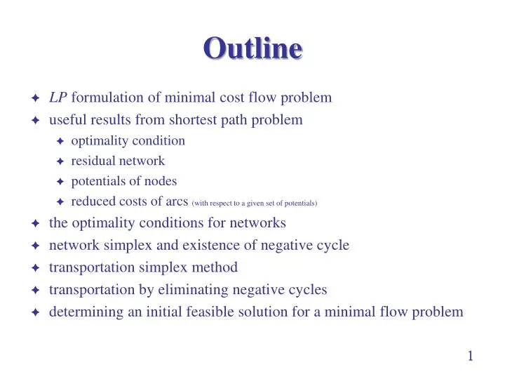
Outline • LP formulation of minimal cost flow problem • useful results from shortest path problem • optimality condition • residual network • potentials of nodes • reduced costs of arcs (with respect to a given set of potentials) • the optimality conditions for networks • network simplex and existence of negative cycle • transportation simplex method • transportation by eliminating negative cycles • determining an initial feasible solution for a minimal flow problem 1
Minimum Cost Flow Models • G: (connected) network, i.e., G = (N, A) • N: the collection of nodes in G, i.e., N = {j} • A: the collection of arcs in G, i.e., A = {(i, j)} • cij: the cost of arc (i, j) • uij:the capacity of arc (i, j) • b(i): the amount of flow out of node i • b(i) > (resp. <) 0 for out (resp. in) flow How to deal with an undirected arc? Assume direct arcs. 2
Minimum Cost Flow Models (cij, uij) • N = {1, 2, 3, 4, 5, 6} • A= {(1, 2), (1, 3), (2, 3), (2, 4), (2, 5), (3, 5), (4, 6), (5, 4), (5, 6)} • b(1) = 9, b(6)= -9, and b(i) = 0 for i = 2 to 5 (5, 7) 2 4 (3, 5) (3, 8) (2, 2) (2, 3) -9 6 1 (5, 4) 9 (4, 6) (2, 3) (4, 3) 3 5 3
A Minimum Cost Flow LP Model (5, 7) 2 4 (3, 5) (3, 8) (2, 2) (2, 3) -9 6 1 (5, 4) 9 (4, 6) (2, 3) (4, 3) 3 5 4
Useful Results from Shortest-Path Algorithms • optimality condition for shortest distances • residual network • potentials of nodes • reduced costs of arcs with respect to a given set of potentials 6
Optimality Condition for Shortest Distances • Theorem. Let G = (N, A) be a directed graph; d() be a function defined on N. Then d() is the shortest distance of node () from node 1 iff • d(1) = 0; • d(i) is the length of a path from node 1 to node i; and • d(j) d(i) + cij for all (i, j) A. 7
Optimality Condition for Shortest Distances • LHS figure: {d(i)} = {0, 2, 3, 7} • for all i, d(i) being shortest distance of node i from node 1 • satisfying the three conditions • RHS figure: {d(i)} = {0, 2, 3, 8} • d(4) = the distance of a path from node 1 to node 4 • d(3) + c34 < d(4), i.e., this set cannot be the collection of shortest distances from nodes d(2) = 2 d(2) = 2 2 2 6 6 2 2 d(4) = 7 d(4) = 8 d(1) = 0 d(1) = 0 1 1 4 4 1 1 4 4 7 7 3 3 d(3) = 3 d(3) = 3 8
1 s t Residual Network (2, 7) (8, 5) 1 s t (2,7) (6, 4) (8,5) Figure 3. The Residual Network Corresponding to Figure 1 (6,4) Figure 1. Costs and Capacities of Arcs (2, 4) (8, 2) 1 1 3 3 3 3 (-8,3) t 0 (-2, 3) s s t (6, 4) Figure 2. Flows on arcs Figure 4. The Residual Network Corresponding to Figure 2 9
t s 1 A Cycle in a Residual Network • actual meaning of sending flow in cycle s-t-1-s(Figure 4) • a different way to send flow from s to t • flow along t-1-s reduction of flow in s-1-t (2, 7) (8, 5) (2, 4) (8, 2) 1 1 0 0 (-6, 3) 3 3 (-8,3) t 3 s (-2, 3) s t (6, 1) Figure 6. Flows on arcs (6, 4) Figure 4. The Residual Network Corresponding to Figure 2 Figure 5. The New Residual Network After Adding a Flow of 3 units in cycle s-t-1-s 10
Potentials of Nodes and the Corresponding Reduced Costs of Arcs • first the idea • call any arbitrary set of numbers {i}, one for a each node, a set of potentials of nodes • define the reduced cost with respect to this set of potentials {i} by • interesting properties for this set of reduced costs 11
Potentials of Nodes and the Corresponding Reduced Costs of Arcs • C(P) be the total cost of path P • C(P) be the total reduced cost of path P • i = potential of node i • P = a path from node s to node t • then C(P) = C(P) s + t 12
Potentials of Nodes and the Corresponding Reduced Costs of Arcs • C(P) be the total cost of path P • C(P) be the total reduced cost of path P • i = potential of node i • P = a path from node s to node t, then • C(P) = C(P) s + t • a shortest path from s to t for C() is also a shortest path from s to t for C() C(P) C(P) 18 2 = -5 4 = 6 2 4 7 4 0 2 4 5 8 4 13 10 6 = 5 1 = 3 6 1 2 4 3 6 1 14 2 -2 3 5 6 3 3 13 3 5 5 = -3 3 = 2
Potentials of Nodes and the Corresponding Reduced Costs of Arcs • C(P) be the total cost of path P • C(P) be the total reduced cost of path P • i = potential of node i • P = a path from node s to node t, then • if j = -d(j), then for all (i, j) A • arcs with forming a tree j = -d(j) 2 = -8 4 = -10 5 2 4 3 0 6 = -12 1 = 0 4 0 8 6 1 0 0 0 3 5 5 = -6 3 = -3 2 = -5 4 = 6 7 2 4 5 8 6 = 5 1 = 3 2 4 3 6 1 6 3 3 14 3 5 5 = -3 3 = 2
Spanning Tree and BFS • in a minimal cost flow network problem, a BFS a spanning tree of the network • # of constraints = # of nodes • # of basic variables = # of nodes - 1 15
The Optimality Conditions for Networks • Theorem 1. (Theorem 9.1, Negative Cycle Optimality Conditions) A feasible solution x* is optimal iff there is no negative cost (direct) cycle in the corresponding residual network G(x*). • Theorem 2. (Theorem 9.3, Reduced Cost Optimality Conditions) A feasible solution x* is optimal iff there exists dual variable such that for every arc (i, j) in the residual network G(x*). • Theorem 3. (Theorem 9.4, Complementary Slackness Optimality Conditions) A feasible solution x* is optimal iff there exists dual variables such that • if then = 0; • if 0 < < uij, then • if then = uij. 17
Ideas for Theorem 1 • a cycle in a residual network: a different way to send flow across a network • existing of a negative cycle existence of another flow pattern with lower cost • no negative cycle no other flow pattern with lower cost 18
Ideas for Theorem 3 • Theorem 3. (Theorem 9.4, Complementary Slackness Optimality Conditions) A feasible solution x* is optimal iff there exists dual variables such that • optimality conditions of simplex method for bounded variables 19
Ideas for Theorem 2 • contradictory statements of Theorem 2 & Theorem 3? • Theorem 2: all reduced costs non-negative (for minimization) • Theorem 3: some reduced costs positive, some negative • Theorem 2: on reduced costs for (variables representing) arcs of a residual network • Theorem 3: on reduced costs of all variables 20
Ideas for Theorem 2 • Theorem 2. (Theorem 9.3, Reduced Cost Optimality Conditions) A feasible solution x* is optimal iff there exists dual variable such that for every arc (i, j) in the residual network G(x*). • Theorem 2 minimum • for any potential and cycle:C(P) = C(P) • for every arc in G(x) no negative cycle in G minimal 21
Ideas for Theorem 2 • Theorem 2. (Theorem 9.3, Reduced Cost Optimality Conditions) A feasible solution x* is optimal iff there exists dual variable such that for every arc (i, j) in the residual network G(x*). • minimum Theorem 2 • conditions of Theorem 3 satisfied by a minimum solution • a forward arc (i, j) with by Theorem 3 • no reversed arc in G(x*) • a forward arc (i, j) with = uij, in the original network • no such forward arc in G(x*) • for the reversed arc in G(x*): • a forward arc (i, j) with in the original network • for the forward arc in G(x*): • for the reversed arc in G(x*): 22
Equivalence Between Network Simplex and Negative Cost Cycle 23
Equivalence Between Network Simplex Method and Existence of a Negative Cost Cycle (cij, uij) • at a certain point, an extended basic feasible solution is shown below, where the dotted lines show arcs at upper bounds. (5, 7) 2 4 (3, 5) (3, 8) (2, 2) (2, 3) -9 6 1 (5, 4) 9 (4, 6) (2, 3) (4, 3) 3 5 Flow 5 2 4 5 7 2 0 0 -9 6 1 9 4 2 2 3 5 24
An Iteration of the Network Simplex • to find the entering variable • x46 entering • reduction of flow from upper bound dual variables 2 = 1 – c12 = -3 4 =-8 5 2 4 Flow 5 3 2 4 1 = 0 How about (2, 3), (2, 5), (5, 4)? 5 7 6 1 2 0 0 -9 6 1 9 6 =-10 4 2 4 3 5 4 2 2 3 5 5 =-6 3 =-2 beneficial to reduce flow in (4, 6) 25
An Iteration of the Network Simplex • to find the leaving variable • reduction of flow from x46 • leaving variable, x13 or x35, for = 1 (5, 7) 2 4 (3, 5) (3, 8) (2, 2) (2, 3) -9 6 1 (5, 4) Change of Flow 9 0 5 7 2 4 (4, 6) (2, 3) (4, 3) 0 5 5 0 7 8 3 5 Current Flow Pattern 0 0 6 5 1 2 4 5 7 0 4+ 6 0 2+ 3 0 2+ 3 3 5 2 0 0 -9 6 1 9 4 2 2 3 5 (cij, uij) 26
An Iteration of the Network Simplex • = 1 • arbitrarily making x35 leaving (5, 7) 2 4 (3, 5) (3, 8) (2, 2) (2, 3) -9 6 1 (5, 4) Change of Flow 9 0 5 7 2 4 (4, 6) (2, 3) (4, 3) 0 5 5 0 7 8 3 5 New Flow Pattern 0 0 6 4 1 2 4 4 6 0 4+ 6 0 2+ 3 0 2+ 3 3 5 2 0 0 -9 6 1 9 5 3 3 3 5 (cij, uij) 27
An Iteration of the Negative Cycle Algorithm • negative cycle 1-3-5-6-4-2-1 • cost = -1 • maximum allowable flow = 1 unit (5, 7) 2 4 (3, 5) (3, 8) (2, 2) (2, 3) -9 6 1 (5, 4) 9 (4, 6) (2, 3) (4, 3) Residual Network 3 5 Current Flow Pattern (cij, xij) 5 2 4 5 7 2 0 0 -9 6 1 9 4 2 2 3 5 (cij, uij) 28
An Iteration of the Negative Cycle Algorithm • negative cycle 1-3-5-6-4-2-1 • cost = -1 • maximum allowable flow = 1 unit (5, 7) 2 4 (3, 5) (3, 8) (2, 2) (2, 3) -9 6 1 (5, 4) 9 (4, 6) (cij, xij) (2, 3) (4, 3) 3 5 (cij, xij) (cij, uij) 29
Same Result from Network Simplex Method and Negative Cost Cycle residual network (cij, xij) (cij, uij) (5, 7) 2 4 (3, 5) (3, 8) (2, 2) (2, 3) -9 6 1 (5, 4) 9 (4, 6) (2, 3) (4, 3) 3 5 New Flow Pattern 4 2 4 4 6 2 0 0 -9 6 1 9 5 3 3 3 5 30
Transportation Simplex Method • balanced transportation problem • 2 sources, 3 destinations • 5 constraints, with one degree of redundancy • 4 basic variables in a BFS 32
Transportation Simplex Method • four basic variables in a BFS 33
Transportation Simplex Method reduced cost (i, j) = cij – ui– vj 34
Transportation Problem by the Negative Cycle Approach • no more negative cycle • optimal flow: x13 = 100, x14 = 500, x15 = 200, x23 = 300, x24 = 0, x25= 0, • minimum cost = 7600 40
To Find an Initial Feasible Solution • to solve a maximal flow problem 42
To Find an Initial Feasible Solution • to solve a minimum cost flow problem • with x1t = 800, x2t = 300, xts = 1100, xs3 = 400, xs4 = 500, xs5 = 200 as the initial solution of the minimal cost flow problem 43


