Download
1 / 22
220 likes | 235 Vues
This statistical analysis evaluates the impact of a new incentive plan on student absences in a large school. The chi-square tests of goodness of fit and independence are utilized to determine if the plan affected absence distribution and student behavior.

E N D
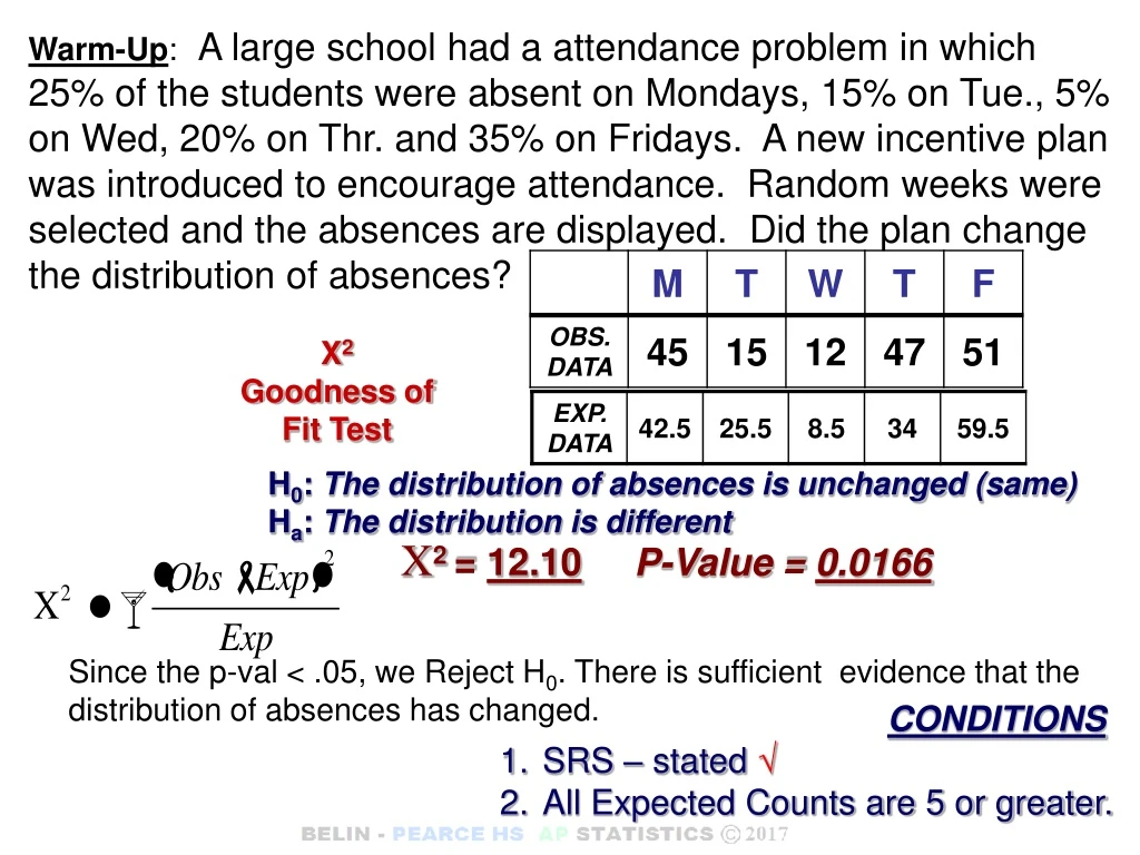
Warm-Up:A large school had a attendance problem in which 25% of the students were absent on Mondays, 15% on Tue., 5% on Wed, 20% on Thr. and 35% on Fridays. A new incentive plan was introduced to encourage attendance. Random weeks were selected and the absences are displayed. Did the plan change the distribution of absences? X2 Goodness of Fit Test H0: The distribution of absences is unchanged (same) Ha: The distribution is different X2 = 12.10 P-Value = 0.0166 Since the p-val < .05, we Reject H0. There is sufficient evidence that the distribution of absences has changed. • CONDITIONS • SRS – stated √ • All Expected Counts are 5 or greater.
9/16 = 0.5625 3/16 = 0.1875 x 100 1/16 = 0.0625
Chapter 26 (continued) The Chi-Square Test of INDEPENDENCE A test of whether TWO categorical variables are independent from each other. In other words, it examines the counts from a sample for evidence of an association between two categorical variables. df = (#Rows – 1) x (#Columns – 1) TWO-WAY TABLES Two way tables are used to show a relationship among two Categorical Variables. Each Cell shows the counts of individuals that fit into both categories.
H0: The two variables are Independent (NO association) Ha: The two variables are NOT Independent (They have a relationship) P-Value = X2cdf (X2, E99, df)
Do Parental smoking habits affect student behavior? 5375 RANDOM students were surveyed. Expected | 332.49 | 1447.51 1780 2239 | 418.22 | 1820.78 1356 | 253.29 | 1102.71 1004 4371 5375 = TT H0: There is NO relationship between Parental smoking habits and student smoking habits. Ha: There is a relationship between Parental smoking habits and student smoking habits. X2 Test of Independence P-Value = X2cdf (37.566, E99, 2) = 0 X2 = 37.566
| 332.49 | 1447.51 | 418.22 | 1820.78 | 253.29 | 1102.71 P-Value = X2cdf (37.566, E99, 2) = 0 X2 = 37.566 Since the P-Value is less than α = 0.05 REJECT H0 . There is a relationship between the smoking habits of Parents and that of students. • CONDITIONS • SRS – stated √ • All Expected Counts are 5 or greater.
EXAMPLE: Some people believe that the full moon elicits unusual behavior in people. The following table shows the number of arrests in a town during weeks of 6 full moons and 6 other randomly selected weeks. Is there evidence that the phase of the moon is associated with degree of the crime?
X2 Test of Independence H0: A Full Moon is independent to the type of crime that is committed. Ha: A Full Moon has an association to the type of crime that is committed. P-Value = X2cdf (2.904, E99, 4) = 0.5740 X2 = 2.904 Since the P-Value is greater than α = 0.05 Fail to REJECT H0 . There is not enough evidence that the full moon has an influence over the types of crimes committed. • CONDITIONS • SRS - Stated √ • All Expected Counts are 5 or greater.X
Chapter 26 - The Chi-Square Test of INDEPENDENCE EXAMPLE: The following example examines the relationship between the Drug treatment and Relapse status for an SRS of chronic cocaine users seeking help to stay off cocaine. H0: Drug treatment is independent of a patient relapses or not. Ha: There is an association of drug treatment to end result. Not all treatments have the same result.
Expected To carry out the significance test with a two table you must calculate the Expected Values. | 16 | 8 24 | 16 | 8 24 | 16 | 8 24 48 24 72 = TT
X2 Test of Independence H0: Drug treatment independent to whether a patient relapses or not. Ha: There is an association of drug treatment to end result. Not all treatments have the same result. P-Value = X2cdf (10.5, E99, 2) = 0.0052 X2 = 10.5 Since the P-Value is less than α = 0.05 the data IS significant . There is strong evidence to REJECT H0 . There is strong evidence that suggests that the drug treatment is associated to relapse. (The treatments differ in terms of their effect.) • CONDITIONS • SRS - Stated √ • All Expected Counts are 1 or greater.√ • No more than 20% of the Expected Counts are less than 5. √
WARM-UP:According to the Statistical Abstract of the US, 1997 the marital status distribution of the US adult population was as follows: 23.26% Never Married, 60.31% Married, 7% Widowed, and 9.43% Divorced. An SRS of 500 US Males, aged 25-29, yielded the following frequency Distribution: Is there evidence the distribution of marital status among males of that Age differs from the US adult population? X2 Goodness of Fit Test H0: The Distribution of Marital Status of US Males age 25-29 is equal to that of all US adults. Ha: The Distribution of Marital Status of US Males age 25-29 is NOT equal to that of all US adults. P-Value = X2cdf (250.24, E99, 3) = 0 X2 = 250.24 Conclusion???
Since the P-Value is less than α = 0.05 the data IS significant . There is strong evidence to REJECT H0 . The Distribution of Marital Status of US Males age 25-29 is Not equal to the that of all US adults. • CONDITIONS • SRS – stated • All Expected Counts are 1 or greater. • No more than 20% of the Expected Counts are less than 5.
EXAMPLE:To determine whether or not Data is Approximately Normal we have examined Bell shaped Curves in Histograms and Symmetry in Box Plots. You can also use a Chi-Squared GOF Test with the 68% - 95% - 99.7% Rule. Determine whether the test scores are Appr. Normally Distributed. TEST Scores 68% 95% 99.7% .34 .34 .135 .135 .025 .025 - ∞ 62.4 76.1 89.8 103.5 117.2 ∞
H0: The data follows an approximately Normal Distribution Ha: The data does NOT follows an approximately Normal Distribution X2 Goodness of Fit Test P-Value = X2cdf (14.599, E99, 5) = 0.0122 X2 = 14.599 Since the P-Value is less than α = 0.05 the data IS significant . There is STRONG evidence to REJECT H0 . The data is NOT approximately Normal. • CONDITIONS • SRS X • All Expected Counts are 1 or greater. X • No more than 20% of the Expected Counts are less than 5. X
Warm-Up:You suspect that a die at a casino craps table has been switched out with a weighted die by a cheating gambler. Based on the following results, is the die in question fair? X2 Goodness of Fit Test H0: The Die is Fair! Ha: The Die is NOT Fair. P-Value = X2cdf (12.75, E99, 5) = 0.0258 X2 = 12.75
Since the P-Value is less than α = 0.05 REJECT H0 . There is strong evidence that the die is weighted. • CONDITIONS • SRS – randomly tossed • All Expected Counts are 1 or greater. • No more than 20% of the Expected Counts are less than 5.