Radiometer Systems
Radiometer Systems. microware remote sensing S. Cruz Pol. Tx. Rx. Rx. Microwave Sensors. Radar (active sensor). Radiometer (passive sensor). Radiometers. Radiometers are very sensitive receivers that measure thermal electromagnetic emission (noise) from material media.


Radiometer Systems
E N D
Presentation Transcript
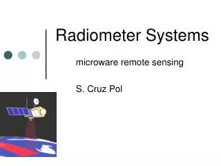
Radiometer Systems microware remote sensing S. Cruz Pol
Tx Rx Rx Microwave Sensors Radar (active sensor) Radiometer (passive sensor) UPR, Mayagüez Campus
Radiometers • Radiometers are very sensitive receivers that measure thermal electromagnetic emission (noise) from material media. • The design of the radiometer allows measurement of signals smaller than the noise introduced by the radiometer (system’s noise). UPR, Mayagüez Campus
Topics of Discussion • Equivalent Noise Temperature • Noise Figure & Noise Temperature • Cascaded System • Noise for Attenuator • Super-heterodyne Receiver • System Noise Power at Antenna • Radiometer Operation • Measurement Accuracy and Precision • Effects of Rx Gain Variations UPR, Mayagüez Campus
Topics of Discussion (cont.) • Dicke Radiometer • Balancing Techniques • Reference -Channel Control • Antenna-Channel Noise-Injection • Pulse Noise-Injection • Gain-Modulation • Automatic-Gain Control (AGC) • Noise-Adding radiometer • Practical Considerations &Calibration Techniques UPR, Mayagüez Campus
TA’ TA Radiometer TB Vout Radiometer’s Task: Measure antenna temperature, TA’ which is proportional to TB, with sufficient radiometric resolution and accuracy • TA’ varies with time. • An estimate of TA’ is found from • Vout and • the radiometer resolution DT. UPR, Mayagüez Campus
Noise voltage • The noise voltage is • the average=0 and the rms is UPR, Mayagüez Campus
Noisy resistor connected to a matched loadis equivalent to… [ZL=(R+jX)*=R-jX] UPR, Mayagüez Campus
B, G radiometer TA Pn=k B G TA TA =200K B, G radiometer Pn=k B G (TA + TN) TN =800K • Ideal radiometer • “Real” radiometer Usually we want DT=1K, so we need B=100MHz and t =10msec UPR, Mayagüez Campus
Receiver antenna Ideal Bandpass Filter B, G=1 ZL Equivalent Output Noise Temperature for any noise source TEis defined for any noise source when connected to a matched load. The total noise at the outputis UPR, Mayagüez Campus
Measurement Accuracy and Precision • Accuracy – how well are the values of calibration noise temperature known in the calibration curve of output corresponding to TA‘ . • Precision – smallest change in TA‘ that can be detected by the radiometer output. UPR, Mayagüez Campus
input signal input thermal noise Noise Figure, F Measures degradation of noise through the device • is defined for To=290K (62.3oF!) Total output signal Total output noise Noise introduced by device UPR, Mayagüez Campus
Noise Figure, F • Noise figure is usually expressed in dB • Solving for output noise power UPR, Mayagüez Campus
Equivalent input noise TE • Noise due to device is referred to the input of the device by definition: • So the effective input noise temp of the device is • Where, to avoid confusion, the definition of noise has been standardized by choosing To=290K (room temperature) UPR, Mayagüez Campus
Cascade System UPR, Mayagüez Campus
Noise for an Attenuator UPR, Mayagüez Campus
Superheterodyne receiver G=23dB F=7.5dB RF amp Grf ,Frf ,Trf IF amp Gif ,Fif ,Tif Mixer LM,FM,TM Pni Pno G=30dB F=2.3dB G=30dB F=3.2dB LO Trf=290(10.32-1)=638K Tm=1,340K Tif=203K UPR, Mayagüez Campus
Total Power Radiometer Super-heterodyne receiver: uses a mixer, L.O. and IF to down-convert RF signal. UPR, Mayagüez Campus
Detection UPR, Mayagüez Campus
IF Noise voltage after IF amplifier UPR, Mayagüez Campus
IF x2 square-law detector represents the average value or dc, and sd represents the rms value of the ac component or the uncertainty of the measurement. Noise voltage after detector UPR, Mayagüez Campus
Low-pass t, gLF x2 integrator Noise voltage after Integrator • Integrator (low pass filter) averages the signal over an interval of time t. • Integration of a signal with bandwidth B during that time, reduces the variance by a factor N=Bt, where B is the IF bandwidth. UPR, Mayagüez Campus
Low-pass t, gLF x2 integrator Radiometric Resolution, DT • The output voltage of the integrator is related to the average input power, Psys UPR, Mayagüez Campus
Receiver Gain variations • Noise-caused uncertainty • Gain-fluctuations uncertainty • Total rms uncertainty • Example p.368 • T’Rec=600K • T’A=300K • B=100MHz • =0.01sec Find the radiometric resolution, DT UPR, Mayagüez Campus
Dicke Radiometer Noise-Free Pre-detection Section Gain = G Bandwidth = B • Dicke Switch • Synchronous Demodulator UPR, Mayagüez Campus
Dicke Radiometer The output voltage of the low pass filter in a Dicke radiometer looks at reference and antenna at equal periods of time with the minus sign for half the period it looks at the reference load (synchronous detector), so The receiver noise temperature cancels out and the total uncertainty in T due to gain variations is UPR, Mayagüez Campus
Dicke radiometer • The uncertainty in T due to noise when looking at the antenna or reference (half the integration time) • Unbalanced Dicke radiometer resolution UPR, Mayagüez Campus
Balanced Dicke A balanced Dicke radiometer is designed so that TA’= Tref at all times. In this case, UPR, Mayagüez Campus
Balancing Techniques • Reference Channel Control • Antenna Noise Injection • Pulse Noise Injection • Gain Modulation • Automatic Gain Control UPR, Mayagüez Campus
Reference Channel Control Force T’A= T ref Switch driver and Square-wave generator, fS Pre-detection G, B, TREC’ Vout TA’ Integrator t Synchronous Demodulator Tref Feedback and Control circuit Vc Variable Attenuator at ambient temperature To L TN Noise Source UPR, Mayagüez Campus
Reference Channel Control • TN and To have to cover the range of values that are expected to be measured, TA’ • If 50k<TA’< 300K • Use To= 300K and need cryogenic cooling to achieve TN =50K. • But L cannot be really unity, so need TN < 50K. To have this cold reference load, one can use • cryogenic cooled loads (liquid nitrogen submerged passive matched load) • active “cold” sources (COLDFET). UPR, Mayagüez Campus
Cryogenic-cooled Noise Source • When a passive (doesn’t require output power to work) noise source such as a matched load, is kept at a physical temperature Tp , it delivers an average noise power equal to kTpB • Liquid N2 boiling point = 77.36°K • Used on ground based radiometers, but not convenient for satellites and airborne systems. UPR, Mayagüez Campus
Active “cold or hot” sources • http://www.maurymw.com/ • http://sbir.gsfc.nasa.gov/SBIR/successes/ss/5-049text.html UPR, Mayagüez Campus
Active noise source-FET • The power delivered by a noise source is characterized using the ENR=excess noise ratio where TNis the noise temperature of the source and To is its physical temperature. • Example for 9,460K , ENR= 15 dB UPR, Mayagüez Campus
Switch driver and Square-wave generator, fS TA” TA’ Vout Pre-detection G, B, Trec’ Coupler Integrator t Synchronous Demodulator Tref L Feedback and Control circuit Vc TN Noise Source Antenna Noise Injection Force T’A= T ref = T o T’N Variable Attenuator Fc = Coupling factor of the directional coupler UPR, Mayagüez Campus
Antenna Noise Injection • Combining the equations and solving for L from this equation, we see that Toshould be>TA’ • If the control voltage is scaled so that Vc=1/L, then Vcwill be proportional to the measured temperature, UPR, Mayagüez Campus
Antenna Noise Injection • For expected measured values between 50K and 300K, Tref is chosen to be To=310K, so • Since the noise temperature seen by the input switch is always To , the resolution is UPR, Mayagüez Campus
Example UPR, Mayagüez Campus
Pulse Noise Injection Switch driver and Square-wave generator, fS TA” TA’ Vout Pre-detection G, B, Trec’ Coupler Integrator t Synchronous Demodulator TN’ Tref Feedback and Control circuit f r Pulse- Attenuation Diode switch Noise Source TN UPR, Mayagüez Campus
tp tR TN’ Diode switch TN Pulse Noise Injection Pulse repetition frequency = fR = 1/tR Pulse width = tp Square-wave modulator frequency fS< fR/2 Switch ON – minimum attenuation Switch Off – Maximum attenuation Example: For Lon = 2, Loff = 100 , To = 300K and T’N = 1000K We obtain Ton= 650K, Toff= 297K UPR, Mayagüez Campus
Pulse Noise Injection • Reference T is controlled by the frequency of a pulse • The repetition frequency is given by For Toff = To, is proportional to T’A UPR, Mayagüez Campus
Automatic-Gain-Control AGC • Feedback is used to stabilize Receiver Gain • Use sample-AGC not continuous-AGC since this would eliminate all variations including those from signal, TA’. • Sample-AGC: Voutis monitored only during half-cycles of the Dicke switch period when it looks at the reference load. • Hach in 1968 extended this to a two-reference-temperature AGC radiometer, which provides continuous calibration. This was used in RadScat on board of Skylab satellite in 1973. UPR, Mayagüez Campus
Dicke Switch • Two types • Semiconductor diode switch, PIN • Ferrite circulator • Switching rate, fS , • High enough so that GS remains constant over one cycle. • To satisfy sampling theorem, fS >2BLF (Same as saying that Integration time is t =1/2BLF) http://envisat.esa.int/instruments/mwr/descr/charact.html UPR, Mayagüez Campus
Dicke Input Switch Two important properties to consider • Insertion loss • Isolation • Switching time • Temperature stability http://www.erac.wegalink.com/members/DaleHughes/MyEracSite.htm UPR, Mayagüez Campus
Radiometer Receiver Calibration • Most are linear systems • The radiometer is connected to two known loads, one cold (usually liquid N2), one hot. • Solve for a and b. • Cold load :satellites • use outer space ~2.7K UPR, Mayagüez Campus
Imaging Considerations • Scanning configurations • Electronic (beam steering) • Phase-array (uses PIN diode or ferrite phase-shifters, are expensive, lossy) • Frequency controlled • Mechanical (antenna rotation or feed rotation) • Cross-track scanning • Conical scanning (push-broom) has less variation in the angle of incidence than cross-track UPR, Mayagüez Campus
Uncertainty Principle for radiometers • For a given integration time, t, there is a trade-off between • spectral resolution, B and • radiometric resolution, DT • For a stationary radiometer, make t larger. • For a moving radiometer, t is limited since it will also affect the spatial resolution. (next) UPR, Mayagüez Campus
Airborne scanning radiometer UPR, Mayagüez Campus
Airborne scanning Consider a platform at height h, moving at speed u, antenna scanning from angles qs and –qs , with beamwidth b, along-track resolution, Dx • The time it takes to travel one beamwidth in forward direction is • The angular scanning rate is • The time it takes to scan through one beamwidth in the transverse direction is the dwell time UPR, Mayagüez Campus
Dwell time • Is defined as the time that a point on the ground is observed by the antenna beamwidth. Using • For better spatial resolution, small t • For better radiometric resolution, large t • As a compromise, choose UPR, Mayagüez Campus