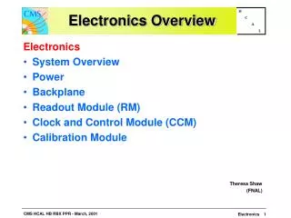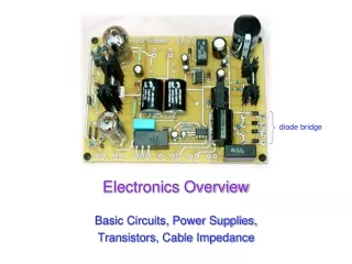
Electronics Overview
Electronics Overview. diode bridge. Basic Circuits, Power Supplies, Transistors, Cable Impedance. Basic Circuit Analysis. What we won’t do: common electronics-class things: RLC, filters, detailed analysis What we will do: set out basic relations

Electronics Overview
E N D
Presentation Transcript
Electronics Overview diode bridge Basic Circuits, Power Supplies, Transistors, Cable Impedance
UCSD: Physics 121; 2012 Basic Circuit Analysis • What we won’t do: • common electronics-class things: RLC, filters, detailed analysis • What we will do: • set out basic relations • look at a few examples of fundamental importance (mostly resistive circuits) • look at diodes, voltage regulation, transistors • discuss impedances (cable, output, etc.)
UCSD: Physics 121; 2012 The Basic Relations • V is voltage (volts: V); I is current (amps: A); R is resistance (ohms: ); C is capacitance (farads: F); L is inductance (henrys: H) • Ohm’s Law: V = IR; V = ; V = L(dI/dt) • Power: P = IV = V2/R = I2R • Resistors and inductors in series add • Capacitors in parallel add • Resistors and inductors in parallel, and capacitors in series add according to:
UCSD: Physics 121; 2012 1 3 2 Example: Voltage divider • Voltage dividers are a classic way to set a voltage • Works on the principle that all charge flowing through the first resistor goes through the second • so V R-value • provided any load at output is negligible: otherwise some current goes there too • So Vout = V(R2/(R1 + R2)) • R2 here is a variable resistor, or potentiometer, or “pot” • typically three terminals: R12 is fixed, tap slides along to vary R13 and R23, though R13 + R23 = R12 always R1 Vout V R2
UCSD: Physics 121; 2012 Real Batteries: Output Impedance • A power supply (battery) is characterized by a voltage (V) and an output impedance (R) • sometimes called source impedance • Hooking up to load: Rload, we form a voltage divider, so that the voltage applied by the battery terminal is actually Vout = V(Rload/(R+Rload)) • thus the smaller R is, the “stiffer” the power supply • when Vout sags with higher load current, we call this “droop” • Example: If 10.0 V power supply droops by 1% (0.1 V) when loaded to 1 Amp (10 load): • internal resistance is 0.1 • called output impedance or source impedance • may vary with load, though (not a real resistor) R V D-cell example: 6A out of 1.5 V battery indicates 0.25 output impedance
UCSD: Physics 121; 2012 A’ A CT B B’ Power Supplies and Regulation • A power supply typically starts with a transformer • to knock down the 340 V peak-to-peak (120 V AC) to something reasonable/manageable • We will be using a center-tap transformer • (A’ B’) = (winding ratio)(A B) • when A > B, so is A’ > B’ • geometry of center tap (CT) guarantees it is midway between A’ and B’ (frequently tie this to ground so that A’ = B’) • note that secondary side floats: no ground reference built-in AC input AC output
UCSD: Physics 121; 2012 I I I I V V V V Diodes • Diodes are essentially one-way current gates • Symbolized by: • Current vs. voltage graphs: acts just like a wire (will support arbitrary current) provided that voltage is positive 0.6 V plain resistor diode idealized diode WAY idealized diode the direction the arrow points in the diode symbol is the direction that current will flow current flows no current flows
UCSD: Physics 121; 2012 Diode Makeup • Diodes are made of semiconductors (usually silicon) • Essentially a stack of p-doped and n-doped silicon to form a p-n junction • doping means deliberate impurities that contribute extra electrons (n-doped) or “holes” for electrons (p-doped) • Transistors are n-p-n or p-n-p arrangements of semiconductors p-type n-type
UCSD: Physics 121; 2012 LEDs: Light-Emitting Diodes • Main difference is material is more exotic than silicon used in ordinary diodes/transistors • typically 2-volt drop instead of 0.6 V drop • When electron flows through LED, loses energy by emitting a photon of light rather than vibrating lattice (heat) • LED efficiency is 30% (compare to incandescent bulb at 10%) • Must supply current-limiting resistor in series: • figure on 2 V drop across LED; aim for 1–10 mA of current
UCSD: Physics 121; 2012 Getting DC back out of AC • AC provides a means for us to distribute electrical power, but most devices actually want DC • bulbs, toasters, heaters, fans don’t care: plug straight in • sophisticated devices care because they have diodes and transistors that require a certain polarity • rather than oscillating polarity derived from AC • this is why battery orientation matters in most electronics • Use diodes to “rectify” AC signal • Simplest (half-wave) rectifier uses one diode: input voltage AC source load diode only conducts when input voltage is positive voltage seen by load
UCSD: Physics 121; 2012 Doing Better: Full-wave Diode Bridge • The diode in the rectifying circuit simply prevented the negative swing of voltage from conducting • but this wastes half the available cycle • also very irregular (bumpy): far from a “good” DC source • By using four diodes, you can recover the negative swing: B & C conduct input voltage A B AC source A & D conduct load C D voltage seen by load
UCSD: Physics 121; 2012 Full-Wave Dual-Supply • By grounding the center tap, we have two opposite AC sources • the diode bridge now presents + and voltages relative to ground • each can be separately smoothed/regulated • cutting out diodes A and D makes a half-wave rectifier AC source A B voltages seen by loads + load C D load can buy pre-packaged diode bridges
UCSD: Physics 121; 2012 Smoothing out the Bumps • Still a bumpy ride, but we can smooth this out with a capacitor • capacitors have capacity for storing charge • acts like a reservoir to supply current during low spots • voltage regulator smoothes out remaining ripple A B capacitor AC source load C D
UCSD: Physics 121; 2012 V C R How smooth is smooth? • An RC circuit has a time constant = RC • because dV/dt = I/C, and I = V/R dV/dt = V/RC • so V is V0exp(t/) • Any exponential function starts out with slope = Amplitude/ • So if you want < 10% ripple over 120 Hz (8.3 ms) timescale… • must have = RC > 83 ms • if R = 100 , C > 830 F
UCSD: Physics 121; 2012 Vin 1 R1 3 2 Vout Rload R2 Regulating the Voltage • The unregulated, ripply voltage may not be at the value you want • depends on transformer, etc. • suppose you want 15.0 V • You could use a voltage divider to set the voltage • But it would droop under load • output impedance R1 || R2 • need to have very small R1, R2 to make “stiff” • the divider will draw a lot of current • perhaps straining the source • power expended in divider >> power in load • Not a “real” solution • Important note: a “big load” means a small resistorvalue: 1 demands more current than 1 M
UCSD: Physics 121; 2012 Vin R1 Vout = Vz Rload Z The Zener Regulator • Zener diodes break down at some reverse voltage • can buy at specific breakdown voltages • as long as somecurrent goes through zener, it’ll work • good for rough regulation • Conditions for working: • let’s maintain some minimal current, Iz through zener (say a few mA) • then (Vin Vout)/R1 = Iz + Vout/Rload sets the requirement on R1 • because presumably all else is known • if load current increases too much, zener shuts off (node drops below breakdown) and you just have a voltage divider with the load zener voltage high slope is what makes the zener a decent voltage regulator
UCSD: Physics 121; 2012 Voltage Regulator IC note zeners • Can trim down ripply voltage to precise, rock-steady value • Now things get complicated! • We are now in the realm of integrated circuits (ICs) • ICs are whole circuits in small packages • ICs contain resistors, capacitors, diodes, transistors, etc.
UCSD: Physics 121; 2012 Voltage Regulators • The most common voltage regulators are the LM78XX (+ voltages) and LM79XX ( voltages) • XX represents the voltage • 7815 is +15; 7915 is 15; 7805 is +5, etc • typically needs input > 3 volts above output (reg.) voltage • A versatile regulator is the LM317 (+) or LM337 () • 1.2–37 V output • Vout = 1.25(1+R2/R1) + IadjR2 • Up to 1.5 A • picture at right can go to 25 V • datasheetcatalog.com for details beware that housing is not always ground
UCSD: Physics 121; 2012 C B E Transistors • Transistors are versatile, highly non-linear devices • Two frequent modes of operation: • amplifiers/buffers • switches • Two main flavors: • npn (more common) or pnp, describing doping structure • Also many varieties: • bipolar junction transistors (BJTs) such as npn, pnp • field effect transistors (FETs): n-channel and p-channel • metal-oxide-semiconductor FETs (MOSFETs) • We’ll just hit the essentials of the BJT here • MOSFET in later lecture E B C pnp npn
UCSD: Physics 121; 2012 Vcc Rc Rb out C in B E BJT Amplifier Mode • Central idea is that when in the right regime, the BJT collector-emitter current is proportional to the base current: • namely, Ice = Ib, where (sometimes hfe) is typically ~100 • In this regime, the base-emitter voltage is ~0.6 V • below, Ib = (Vin 0.6)/Rb; Ice =Ib = (Vin 0.6)/Rb • so that Vout = Vcc IceRc = Vcc (Vin 0.6)(Rc/Rb) • ignoring DC biases, wiggles on Vin become (Rc/Rb) bigger (and inverted): thus amplified
UCSD: Physics 121; 2012 Vcc Rc Rb out in Switching: Driving to Saturation • What would happen if the base current is so big that the collector current got so big that the voltage drop across Rc wants to exceed Vcc? • we call this saturated: Vc Ve cannot dip below ~0.2 V • even if Ib is increased, Ic won’t budge any more • The example below is a good logic inverter • if Vcc = 5 V; Rc = 1 k; Ic(sat) 5 mA; need Ib > 0.05 mA • so Rb < 20 k would put us safely into saturation if Vin = 5V • now 5 V in ~0.2 V out; < 0.6 V in 5 V out
UCSD: Physics 121; 2012 Vcc in out R Transistor Buffer • In the hookup above (emitter follower), Vout = Vin 0.6 • sounds useless, right? • there is no voltage “gain,” but there iscurrent gain • Imagine we wiggle Vin by V: Vout wiggles by the same V • so the transistor current changes by Ie = V/R • but the base current changes 1/ times this (much less) • so the “wiggler” thinks the load is V/Ib = ·V/Ie = R • the load therefore is less formidable • The “buffer” is a way to drive a load without the driver feeling the pain (as much): it’s impedance isolation
UCSD: Physics 121; 2012 Vin Vin Rz Vz Vreg Z Rload Improved Zener Regulator • By adding a transistor to the zener regulator from before, we no longer have to worry as much about the current being pulled away from the zener to the load • the base current is small • Rload effectively looks times bigger • real current supplied through transistor • Can often find zeners at 5.6 V, 9.6 V, 12.6 V, 15.6 V, etc. because drop from base to emitter is about 0.6 V • so transistor-buffered Vreg comes out to 5.0, 9.0, etc. • Iz varies less in this arrangement, so the regulated voltage is steadier
UCSD: Physics 121; 2012 Switching Power Supplies • Power supplies without transformers • lightweight; low cost • can be electromagnetically noisy • Use a DC-to-DC conversion process that relies on flipping a switch on and off, storing energy in an inductor and capacitor • regulators were DC-to-DC converters too, but lossy: lose P = IV of power for voltage drop of V at current I • regulators only down-convert, but switchers can also up-convert • switchers are reasonably efficient at conversion
UCSD: Physics 121; 2012 Switcher topologies The FET switch is turned off or on in a pulse-width-modulation (PWM) scheme, the duty cycle of which determines the ratio of Vout to Vin from: http://www.maxim-ic.com/appnotes.cfm/appnote_number/4087
UCSD: Physics 121; 2012 Step-Down Calculations • If the FET is on for duty cycle, D (fraction of time on), and the period is T: • the average output voltage is Vout = DVin • the average current through the capacitor is zero, the average current through the load (and inductor) is 1/D times the input current • under these idealizations, power in = power out
UCSD: Physics 121; 2012 Step-down waveforms • Shown here is an example of the step-down with the FET duty cycle around 75% • The average inductor current (dashed) is the current delivered to the load • the balance goes to the capacitor • The ripple (parabolic sections) has peak-to-peak fractional amplitude of T2(1D)/(8LC) • so win by small T, large L & C • 10 kHz at 1 mH, 1000 F yields ~0.1% ripple • means 10 mV on 10 V FET Inductor Current Supply Current Capacitor Current Output Voltage (ripple exag.)
UCSD: Physics 121; 2012 Cable Impedances • RG58 cable is characterized as 50 cable • RG59 is 75 • some antenna cable is 300 • Isn’t the cable nearly zero resistance? And shouldn’t the length come into play, somehow? • There is a distinction between resistance and impedance • though same units • Impedances can be real, imaginary, or complex • resistors are real: Z = R • capacitors and inductors are imaginary: Z = i/C; Z = iL • mixtures are complex: Z = R i/C + iL
UCSD: Physics 121; 2012 Impedances, cont. • Note that: • capacitors become less “resistive” at high frequency • inductors become more “resistive” at high frequency • bigger capacitors are more transparent • bigger inductors are less transparent • i (√1) indicates 90 phase shift between voltage and current • after all, V = IZ, so Z = V/I • thus if V is sine wave, I is cosine for inductor/capacitor • and given that one is derivative, one is integral, this makes sense (slide # 3) • adding impedances automatically takes care of summation rules: add Z in series • capacitance adds as inverse, resistors, inductors straight-up
UCSD: Physics 121; 2012 Impedance Phasor Diagram • Impedances can be drawn on a complex plane, with pure resistive, inductive, and capacitive impedances represented by the three cardinal arrows • An arbitrary combination of components may have a complex impedance, which can be broken into real and imaginary parts • Note that a system’s impedance is frequency-dependent imag. axis Zi Z L Zr real axis R 1/C
UCSD: Physics 121; 2012 Transmission Line Model • The cable has a finite capacitance per unit length • property of geometry and dielectric separating conductors • C/l = 2πε/ln(b/a), where b and a are radii of cylinders • Also has an inductance per unit length • L/l = (μ/2π)ln(b/a) • When a voltage is applied, capacitors charge up • thus draw current; propagates down the line near speed of light • Question: what is the ratio of voltage to current? • because this is the characteristic impedance • Answer: Z0 = sqrt(L/C) = sqrt(L/C) = (1/2π)sqrt(μ/ε)ln(b/a) • note that Z0 is frequency-independent input L output C
UCSD: Physics 121; 2012 Typical Transmission Lines • RG58 coax is abundant • 30 pF per foot; 75 nH per foot; 50 ; v = 0.695c; ~5 ns/m • RG174 is the thin version • same parameters as above, but scaled-down geometry • RG59 • used for video, cable TV • 21 pF/ft; 118 nH per foot; 75 ; v = 0.695c; ~5 ns/m • twisted pair • 110 at 30 turns/ft, AWG 24–28 • PCB (PC-board) trace • get 50 if the trace width is 1.84 times the separation from the ground plane (assuming fiberglass PCB with = 4.5)
UCSD: Physics 121; 2012 Why impedance matters • For fast signals, get bounces (reflections) at every impedance mismatch • reflection amplitude is (Zt Zs)/(Zt + Zs) • s and t subscripts represent source and termination impedances • sources intending to drive a Z0 cable have Zs = Z0 • Consider a long cable shorted at end: insert pulse • driving electronics can’t know about the termination immediately: must charge up cable as the pulse propagates forward, looking like Z0 of the cable at first • surprise at far end: it’s a short! retreat! • in effect, negative pulse propagates back, nulling out capacitors (reflection is 1) • one round-trip later (10 ns per meter, typically), the driving electronics feels the pain of the short
UCSD: Physics 121; 2012 Impedance matters, continued • Now other extreme: cable un-terminated: open • pulse travels merrily along at first, the driving electronics seeing a Z0 cable load • at the end, the current has nowhere to go, but driver can’t know this yet, so keeps loading cable as if it’s still Z0 • effectively, a positive pulse reflects back, double-charging capacitors (reflection is +1) • driver gets word of this one round-trip later (10 ns/m, typically), then must cease to deliver current (cable fully charged) • The goldilocks case (reflection = 0) • if the end of the cable is terminated with resistor with R = Z0, then current is slurped up perfectly with no reflections • the driver is not being lied to, and hears no complaints
UCSD: Physics 121; 2012 So Beware! • If looking at fast (tens of ns domain) signals on scope, be sure to route signal to scope via 50 coax and terminate the scope in 50 • if the signal can’t drive 50 , then use active probes • Note that scope probes terminate to 1 M, even though the cables are NOT 1 M cables (no such thing) • so scope probes can be very misleading about shapes of fast signals
UCSD: Physics 121; 2012 References and Assignment • References: • The canonical electronics reference is Horowitz and Hill: The Art of Electronics • Also the accompanying lab manual by Hayes and Horowitz is highly valuable (far more practically-oriented) • And of course: Electronics for Dogs (just ask Gromit) • Reading • Sections 6.1.1, 6.1.2 • Skim 6.2.2, 6.2.3, 6.2.4 • Sections 6.3.1, 6.5.1, 6.5.2 • Skim 6.3.2