Usefulness of randomization techniques. Monte-Carlo methods. The Bootstrap.

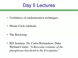
1. Day 5 Lectures • Usefulness of randomization techniques. • Monte-Carlo methods. • The Bootstrap. • IES Seminar: Dr. Curtis Richardson, Duke Wetland Center, "A Bayesian estimate of the phosphorus threshold in the Everglades."

2. Randomization Techniques • When linking models to data, we must estimate model parameters. • Are the parameters “true”? Do they reflect the true mechanisms and processes in the natural world? • We can increase confidence bytesting our methods on data where we know exactly what is going on. • Randomization techniques allow us to perform simulated experiments to draw statistical conclusions about a model and parameter estimates. • Very computer-intensive. B&A 2002

3. Monte-Carlo methods • Population of interest is simulated. • Draw repeated samples from pseudo-population. • Statistic (parameter) computed in each pseudo-sample. • Sampling distribution of statistic examined. • Where do true parameters fall within this distribution?

4. An example….. The Data: xi = measurements of DBH on 50 adult trees yi = measurements of crown radius on those trees The Scientific Model: We generate a dataset with known parameters (a, b) using the model yi = a + b xi + e and randomly generated error term (e). The Probability Model: We generate a normally distributed error e, with mean = 0 and variance d2. Can we recover the true parameter values?

5. Basic procedure • Calculate predicted values with known parameter values. • Add random error to predicted values to create observed. • Estimate parameter values given observed and predicted. • Go back to step 2 and loop through 100-1000 times. • Examine frequency distribution of estimated parameters of interest.

8. Mean of predicted

9. Std. dev. Of error Desired number of observations GENERATE ERRORS

10. Y=observed T=DBH Error + predicted = Observed

11. Residuals = Errors

12. CALCULATE LIKELIHOOD Std. Deviation of residuals

13. Initial parameter estimates Including std dev of residuals ESTIMATE PARAMETERS

15. Parameter for which we want a distribution

16. EXAMINE TRUE PARAMETERS AND RESULTS OF MONTE-CARLO

17. A more interesting example….. The Data: xi = measurements of DBH on 50 adult trees yi = measurements of crown radius on those trees The Scientific Model: We generate a dataset with known parameters (a, b) using the model yi = a + b xi + e and two types or randomly generated error term (e): process error and observation error. The Probability Model: We generate a normally distributed error e, with mean = 0 and variance d2. What is the effect of adding each type of error on parameter estimates?

18. Basic procedure We generate two datasets with known parameters (a, b) using the following error structures: yi = a + b xi + e Process error (e.g., relationship between DBH varies across space, among genotypes). yi = a + b (xi + e)  Observation error (error in measuring DBH)

19. Process error yi = a + b xi + e Process error

20. Observation error: large scatter yi = a + b (xi + e)  Observation error

21. Process vs. observation uncertainty

22. 600 400 200 0 0.5 1.0 1.5 600 400 200 0 0.5 1.0 1.5 2.0 Process and observation uncertainty 600 400 Count 200 0 2.0 0.5 1.0 1.5 2.0 Observation Observation & Process Process Distribution of parameter α for each type of uncertainty.

23. Use of Monte Carlo methods to test assumptions • What is the effect of assuming normal errors -if the errors are lognormally distributed- on parameter estimation? • For process error? • For observation error?

24. Use of Monte Carlo methods to test assumptions:Incorrect assumptions about error distribution yi = a + b xiTrue modela = 1.18 b = 0.07 yi = a + b xi + e Process errora = 1.83 b = 0.06 yi = a + b (xi + e)  Observation error a =1.22 (error in measuring DBH) b = 0.07

25. Things to think about….. • The proper generation of errors is crucial in the success of a Monte-Carlo process because the the random error is what drives the sampling distribution of estimated parameters. • It is usually good practice to standardize generated errors with respect to mean and variance by subtracting from each case the theoretical mean of the generating distribution and dividing by the square root of the theoretical variance. H&M 1997

26. The Bootstrap • Draw conclusions about the population parameter from sample at hand. • Draw repeated sub-samples from population with replacement. • Statistic (parameter) computed in each subsample. • Sampling distribution of statistic examined.

27. An example….. The Data: xi = measurements of DBH on 50 adult trees yi = measurements of crown radius on those trees The Scientific Model: yi = a + b xi + e (linear relationship, with 2 parameters (a, b) and an error term (e) (the residuals)) The Probability Model: e is normally distributed, with mean = 0 and variance estimated from the observed variance of the residuals...

28. Going back to a previous example… The Data: xi = measurements of DBH on 50 adult trees yi = measurements of crown radius on those trees Resample 50 adult trees with replacement. The Scientific Model: yi = a + b xi + e Estimate a and b from each sample. The Probability Model: Examine probability distribution of a and b.

29. Basic procedure • Resample actual data 100-1000 times with replacement. • Estimate parameter values for each resampling. • Examine frequency distribution of estimated parameters of interest.

32. Use parameter estimates to calculate predicted and residuals

33. Calculate likelihood of Bootstrap sample

35. OUTPUT OF BOOTSTRAP FOR PARAMETER A

36. USE SUMMARY STATS TO UNDERSTAND DISTRIBUTION OF PARAMETER ESTIMATE OR TO CALCULATE C.I. S

37. Suggested References • Efron, B. and R.J. Tibshirani. “An introduction to the bootstrap.” Chapman & Hall, London. • “Bootstrapping: A non-parametric approach to statistical inference”. C.Z. Mooney and R.D. Duval. No. 96 of Quantitative Applications in the Social Sciences. Sage University Press. • “Monte Carlo Simulation”. C.Z. Mooney. No. 116 of Quantitative Applications in the Social Sciences. Sage University Press. • “The Ecological Detective: confronting models with data”. R. Hillborn and M. Mangel. Princeton University Press.