Download
1 / 16
160 likes | 386 Vues
1.5 – Linear Functions 1.6 – Linear Regression. 1.5 Slope Intercept Form ( Pg 77). If we write the equation of a linear function in the form. f(x) = b + mx Then m is the slope of the line, and b is the y-intercept. 1.5 Equations of Lines ( Pg 79). y = 2 x + 1. y = 2 x y = ½ x.

E N D
1.5 Slope Intercept Form ( Pg 77) If we write the equation of a linear function in the form. f(x) = b + mx Then m is the slope of the line, and b is the y-intercept
1.5 Equations of Lines ( Pg 79) y = 2x + 1 y = 2x y = ½ x 3 1 -2 y = 2x + 3 y = 2x - 2 y = -2x These lines have the same y- intercept but different slopes These lines have the same slope but different y - intercepts
1.5 Slope – Intercept FormGeneraly = mx + b ( m is slope of a line, and b is the y- intercept) Slope- Intercept Method of Graphing New point x y = mx + b y b Start here
Point- Slope Form ( pg 82 ) 5 x axis Point- Slope Formy = y1 + m (x – x1) y-3 and point ( 1, - 4) x = 4 ( Start point) (1, - 4) - 4 y = -3 ( New Point ) (5, - 7) - 7 x = 4 Plot (1, -4) and move -3 in y-direction and then + 4 in the x-direction to get the new point(5, -7)
1.5 Slope – Intercept Formy = mx + b ( m is slope of a line, and b is the y- intercept) 3x + 4y = 6 (Subtract 3x from both sides) 4y = - 3x + 6 (Divide both sides by 4) y = - 3x + 3 ( Isolate Y, divide by 4 ) 4 2 m = -3 and b = 3 4 2
Ex1.5, 12 a) Pg 85, Sketch the graph of the line with the given slope and y-intercept b) Write an equation for the line c) Find the x-intercept of the line m= - 4 and b = 1 ( 0, 1) 1 -1 -2 -3 -4 Solution (1, - 3) a) Plot y intercept = (0,1) and move - 4 units y-direction down and 1 unit in the x direction( right) to arrive at (1, -3). Draw the line through the two points b) y= 1- 4x ( y = mx + b, equation of line) c) Set y= 0, 0 = 1 – 4x ( y = mx = b, Equation ) 4x = 1 ( Divide by 4 ) x = ( x- intercept)
N0 38a) Write an equation in point slope form for the line that passes through the given point and has the given slopeb) Put your equation from part a) into slope –intercept formc) Use your graphing calculator to graph the line(7.2, - 5.6); m = 1.6Solution a) y = - 5.6 + 1.6(x – 7.2) { Pt. slope form, y = y1 + m (x – x1)} b) Solve the equation for y y = - 5.6 + 1.6(x – 7.2) y = -17.12 + 1.6x (slope intercept form) C) Use Graphing Calculator Hit Y and enter equation Hit window , enter values Hit Graph [-6, 16,1] by [ -20, 6, 1]
Ch 1.6 Scatter Plots ( pg 94 ) scattered not organized decreasing trend increasing trend
1.6 Linear Regression (Lines of Best Fit) • The datas in the scatter plot are roughly linear, we can estimate the location of imaginary ”lines best fit” that passes as close as possible to the data points • We can make the predictions about the data. The process of predicting a value of y based on a straight line that fits the data is called a linear regression, and the line itself called the regression line. • The equation of the regression line is usually used (instead of graph) to predict values
Example of Linear Regression • Estimate a line of best fit and find the equation of the regression line • Use the regression line to predict the heat of vaporization of • potassium bromide, whose boiling temperature is 14350C 200 100 Heat of Vaporization (kJ) (1560, 170) (900, 100) Choose two points in the regression line 1000 2000 Boiling Point 0 C a) Slope = m = 170 – 100 = 0.106 1560 – 900 The equation of regression line is y- y1 = m(x – x1) ( Pt. slope formula) y – 100 = 0.106(x – 900) , y = 0.106x + 4.6 b)Regression equation for potassium bromide , x = 1435 y = 0.106(1435) + 4.6
Interpolation- The process of estimating between known data points Extrapolation- Making predictions beyond the range of known data 112 96 80 64 48 Height (cm) 20 40 60 80 100 Age (months) The graph is not linear because her rate of growth is not constant; her growth slows down as she approaches her adult height. The short time of interval the graph is close to a line, and that line can be used to approximate the coordinates of points on the curve.
Using Graphing Calculator for Linear Regression Pg – 99a) Find the equation of the least square regression line for the following data:( 10, 12), (11, 14), ( 12, 14), (12, 16), ( 14, 20)b) Plot the data points and the least squares regression lin eon the same axes. Step 1Press Stat , choose 1 press Enter Step 2Enter Y = 1.95x – 7.86 Step 4 Press Vars 5 ,Right,Right , Enter Step 3Stat, right arrow go to 4 and enter Step 5Press 2nd, Stat Plot 1 and enter Step 6 Zoom 9
Ex 1.6, Pg - 101No 4. On an international flight, a passenger may check two bags each weighing 70 kg, or 154 pounds, and one carry –on bag weighing 50 kg, or 110 pounds. Express the weight, p, of a bag in pounds in terms of its weight, k, in kilograms Solution a) b) Slope m = 154 – 110 = 44 = 2.2 ( Slope) 70 – 50 20 p = 110 + 2.2 (k – 50) ( pt. slope form ) p = 110 + 2.2k – 110 p = 2.2kg c) m = 2.2 ib/kg is the factor for conversion from kg to pounds
No 14 The number of mobile homes in the United States has been increasing since 1960. The data in the table are given in millions of mobile homes • Let t represent the number of years after 1960 and plot the data. Draw a line • of best fit for the data points • b. Find an equation for your regression line • c. How many mobile homes do you predict for 2010 ? • Solution Use calculator for the b) Linear regression with the points is y = 0.5 + 0.213t, where y represents the number of mobile homes in millions c) 2010 , t = 50 y = 0.5 + 0.213t = 0.5 + 0.213(50) =11.15 11, 150,000 mobile homes in 2010 12 8 4 Consider 1960 as 0 Half of the points above line and half of points below the line (8.8, 40) ( 30, 7.4) (4.7, 20) (2.1, 10) (0, 0.8) 10 20 30 40 50
Graphing Calculator Use page 99 ( Text book) Press Stat Enter to select Edit. Enter the points in L1 and L2 . ( Use the down,up, side arrows), Press Stat side arrow 4 select Lin Reg (ax + b) and press Enter Press Y1 and press VARS 5 and two sides arrows and enter To draw a scatter plot press 2nd Y = 1 and set plot 1 menu then zoom 9