1. Introduction

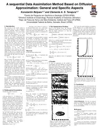
1. UFBA A sequential Data Assimilation Method Based on Diffusion Approximation: General and Specific Aspects Konstantin Belyaev1,2 and Clemente A. S. Tanajura1,3 1Centro de Pesquisa em Geofísica e Geologia (CPGG/UFBA) 2Shirshov Institute of Oceanology, Russian Academy of Sciences (Shirshov) 3Dept. de Física da Terra e do Meio Ambiente, Instituto de Física (IF/UFBA) Universidade Federal da Bahia, Salvador, Brazil (UFBA) . UFBA . 1. Introduction The correction of the model results by observational data by a data assimilation scheme is generally realized as follows. Given a time-interval (to ,T), it can be broken down into subintervals (to , t1), (t 1, t2),..., (tk,tk+1). On any subinterval (tk,tk+1), the model starts at moment tk with the initial vector θk, also called as background state vector, and integrates forward until moment tk+1 , when it produces a new state-vector .Here and further, the superscript m indicates that the system state has been obtained only by model integration without any other source of information. Over the time-interval (tk,tk+1), a series of measurements of the state variable represented by the vectors are taken independently of the model. Then, the model output at time k+1 is corrected by both observational information and the model state taken during the time interval according to the scheme: (*) Here, H denotes the projection of model variables in the model domain onto the observational locations at each subinterval. The model and the measured variables are considered at the moments in which the observational data become available. The weight functions α also depend on time and space and may be either known a priori or determined by some appropriate algorithm. The corrected state-vector, the so-called objective analysis, is now taken as the new initial condition for the next step of the model integration. In spite of substantial differences in the calculation of the weight coefficient, the majority of the data assimilation methods follows the scheme mentioned above. Therefore, here we investigate several general aspects and mathematical properties of this scheme. Also, some numerical applications were performed and few results are presented. 3. The Optimisation Problem Based on the theorem above the following optimization problem can be posed and solved: Find the weight coefficients α so that they minimise the functional under the condition where C is a constant associated with the model bias with respect to observations. The minimisation of this functional leads to α as a solution oftheequations whereΦ is anunknownvectorofLagrangeanmultipliers. 4. Results To show an application ofthemethod in oceanography, themodel MOM4 wasusedalongwithobservational data of vertical profilesoftemperaturefromthe TOGA/TAO array. Fewresults are presentedbelow for theassimilationofdaily data onJanuary 2, 2001 in whichthemodelwasforcedwith NCEP reanalysis. Alldetails are described in Tanajura andBelyaev (2008). Fig. 1 shows themodelsimulation, assimilationandthedifference for 5 m depthtemperatureonJanuary 2, 2001. Fig. 2 shows the vertical profilesoftemperatureattwopoints, one in whichthere is a mooringandtheother in whichtheaverageofneighboormooringslyingwithin a circlewith 1000 km radiuswastaken as anestimateoftheobservations. Knowing (i) the solution of system (1) for the given initial vector on the entire interval ; (ii) the observed variables ; and (iii) the value of the random index νk,n, the newly constrained variables are introduced by the formula (2) In this manner, it becomes possible to constrain the sequence of trajectories of the random process over the entire interval (0,T). Starting from some known random vector , the solution of (2) on each interval Δtk,nwith jumps at the correction time can be evaluated. The limiting behaviour of the trajectories provided by (2) when is here investigated. Theorem Let the following conditions hold: A1. The intervals  0 uniformly with respect to k, i.e., ; A2. The probability distribution for the random variables νk,nsatisfies the conditions for any k, and ; A3. The random vectors have 2+ moments for positive in each series n, i.e., , and these variables are uniformly bounded with respect to n for any k; A4. The operator Λ is a continuous function on its arguments; A5. The set of weight coefficients is uniformly bounded with respect to n; A6. There exists some random variable and the sequence of distributions of random variables converges to the distribution of , i.e., for each x as n. Then, thesequence of finite-dimensional distributions of random processes converges to the distribution of a stochastic process , which will be a solution of the following stochastic differential equation where and The standard Wiener process w(t) is defined on the interval (0,T) and it is independent of the random variable . a) b) Figure 2. Temperature vertical profiles calculated by the model simulation (thin line), assimilation (thick line) and observation (dashed line) at the point (a) (0°N, 180°E); and (b) (2°N, 190°E) on January 2, 2001. Unit is oC. 5. Conclusions The results presented here are of both theoretical and practical interests. From the theoretical point of view, it is important to know: (i) when and under which conditions the solution of differential equations (1) with the correction (2) may be approximated by a continuous function; and (ii) how the limit function can be calculated numerically. From the practical point of view, the scheme can be utilised to determine a variety of relevant parameters, such as a measure of the assimilation quality. Also, the proposed scheme is rather general and, therefore, some popular schemes, such as optimal interpolation, can be considered as special cases. Acknowledgements. This work wasfinanciallysupportedby PETROBRAS and Agência Nacional do Petróleo, Gás Natural e Biocombustíveis(ANP), Brazil, via the Oceanographic Modelling and Observation Research Network (REMO). a) 2. Mathematicalformulation Consider the system of equations (1) on the time-interval (to , T). Without loss of generality, hereafter will be associated with 0, while T may be both finite and infinite. In (1), θ(t) represents the random state-vector of dimension r defined on a given probability space, and Λ(θ, t) denotes a non-random, in general non-linear, operator acting in Rr , which does not explicitly involve temporal derivatives. A sequence of time series is considered, such that for each series the interval (0,T) is broken down by the points The first index in this series denotes time moments in chronological order, and the second index refers to the number of series. It is supposed that in each series on the interval a number of random vectors i=0, 1,… are observed. Here νk,n is a random integer multi-index with the given distribution independent of vectors . b) References Daley, R. Atmospheric Data Anaslysis. Cambridge Univ. Press. 457 pp. (1991) Kalnay, E. AtmosphericModeling, Data AssimilationandPredictability. Cambridge Univ. Press, 341 pp. (2003) Tanajura, C.A.S. and K. Belyaev. On the oceanic impact of a data assimilation method on a coupled ocean-land-atmosphere model. Ocean Dynamics, 52, 123-132 (2002). Tanajura, C.A.S.and K. Belyaev. A sequential data assimilation methodbased on the properties of a diffusion-type process. Applied Mathematical Modelling (in press) (2008) c) Figure 1. (a) MOM4 model simulated 5 m depth temperature field in contour lines and mooring locations marked by shaded circles; (b) assimilated 5 m depth temperature field; (c) difference assimilation minus simulation at 5 m depth temperature. The simulation is for January 2, 2001. Unit is oC.