Modeling VoIP in Cognitive Radio Network
260 likes | 413 Vues
Modeling VoIP in Cognitive Radio Network. Students: Taly Sessler 038741401 Ben Rubovitch 065631475 Instructor: Boris Oklander Semester: Winter 2010. Index. Introduction 1.1 VoIP 1.2 Cognitive Radio 2. Project’s Goals 3. Model Description 4. Simulation design 5. Results

Modeling VoIP in Cognitive Radio Network
E N D
Presentation Transcript
Modeling VoIP in Cognitive Radio Network Students: Taly Sessler 038741401 Ben Rubovitch 065631475 Instructor: Boris Oklander Semester: Winter 2010
Index • Introduction 1.1 VoIP 1.2 Cognitive Radio 2. Project’s Goals 3. Model Description 4. Simulation design 5. Results • Conclusions • Summery
Introduction to VoIP • Voice over Internet Protocol- VoIP is a general term for a family of transmission technologies for delivery of voice communications over IP networks such as the Internet or other packet-switched networks. • Flexibility - VoIP can facilitate tasks and provide services that may be more difficult to implement using the PSTN. • Many telephone calls over a single channel. • Secure calls using standardized protocols. • Location independence. • Integration with other Internet services.
Introduction to VoIPRelevant challenges • Quality of Service – the network cannot ensure that the data packets are delivered in sequential order, or provide Quality of Service (QoS) guarantees, VoIP implementations may face problems mitigating latency and jitter. • Delay Jitter - in the context of computer networks, the term jitter is often used as a measure of the variability over time of the packet latency across a network. • Jitter Buffer - Some systems use sophisticated delay-optimal de-jitter buffers that are capable of adapting the buffering delay to changing network jitter characteristics.
Introduction to VoIP • clustering / dispersion → overflow / time-outs • Trade-offs management: Delay ↔ Loss
Introduction to Cognitive Radio • Cognitive Radio (CR) is a new wireless communication paradigm. • CR characteristics: • Based on Software Defined Radio (SDR). • CR is aware of its environment and use case. • Spectrum Sensing • Spectrum Analysis • Spectrum Decision
Project Goals • Studying VoIP technology with emphasis on Oos aspects • Implementation of VoIP CRNModel usingMATLAB@ • Executing and Performance studying
Network & Codec Jitter Buffer Voice Quality Loss Delay λ K TDelay jitter buffer jitter buffer codec codec codec codec System’s Model E-model R-Factor MOS • Network conditions • Delay • Loss • Codec characteristics • Equipment impairment • Loss robustness jitter buffer controller
Network & Codec Jitter Buffer Voice Quality jitter buffer jitter buffer codec codec codec codec CRN System’s Model E-model R-Factor MOS jitter buffer controller CRN
Network & Codec Jitter Buffer Voice Quality Loss Delay λ K TDelay jitter buffer jitter buffer codec codec codec codec CRN System’s Model E-model R-Factor MOS • Network conditions • Delay • Loss • Codec characteristics • Equipment impairment • Loss robustness C(t) jitter buffer controller
Network Simulator Scenarios generator Network simulator Adaptive Jitter Buffer MOS Channel State Simulator Performance Studying
Channel State Simulator Design Inputs: M – number of channels Ci(t) – state of ith channel i=1,2,…,M PU parameters α,β Simulation time Outputs: Channels(t) – state of channels
Channel State Simulator Design Change 1: for i = 1:Network.channel_set.M nst = find(Network.channels(i).times > slot(n),1)-1; network_state = network_state + Network.channels(i).state(nst); if isempty(network_state) error('1'); end End Change 2: if network_state == 0 Stream.TOA(id) = -1; else Stream.TOA(id) = Stream.TOC(id)+Session.T_packet*50/network_state; if Stream.TOA(id) < Stream.TOA(id-1) Stream.TOA(id) = Stream.TOA(id-1)+ Session.T_packet/10000; end end
Results and Conclusions Jitter Buffer Algorithm Types Analytic - AJB AR-1 – re-evaluation AR-N – re-evaluation Constant Delay
Conclusions • We can see that for each situation there is an algorithm that fits it, but there is no good algorithm for all Network and Participant types. • The use of Algorithm will be done by the state of known factors in the Network and Participant with the use of the tables above
Summery • In this project we integrated a network simulation that fits better with realistic Network. • Upgraded the Jitter Buffer’s algorithm by dumping packets that came later then their successors and simulated a more realistic Time Of Arrival. • Generated a table that covers a vast variety of situations which the Jitter Buffer can choose an algorithm from