Download
1 / 29
290 likes | 411 Vues
Statistics in the Image Domain for Mobile Robot Environment Modeling. L. Abril Torres-Méndez and Gregory Dudek Centre for Intelligent Machines School of Computer Science McGill University. Our Application. Automatic generation of 3D maps. Robot navigation, localization

E N D
Statistics in the Image Domain forMobile Robot Environment Modeling L. Abril Torres-Méndez and Gregory Dudek Centre for Intelligent Machines School of Computer Science McGill University
Our Application • Automatic generation of 3D maps. • Robot navigation, localization - Ex. For rescue and inspection tasks. • Robots are commonly equipped with camera(s) and laser rangefinder. • Would like a full range map of the the environment. • Simple acquisition of data
Problem Context • Pure vision-based methods • Shape-from-X remains challenging, especially in unconstrained environments. • Laser line scanners are commonplace, but • Volume scanners remain exotic, costly, slow. • Incomplete range maps are far easier to obtain that complete ones. • Proposed solution: Combine visual and partial depth Shape-from-(partial) Shape
From range scans like this infer the rest of the map Problem Statement From incomplete range data combined with intensity, perform scene recovery.
Overview of the Method • Approximate the composite of intensity and range data at each point as a Markov process. • Infer complete range maps by estimating joint statistics of observed range and intensity.
far surface smoothness surface smoothness variations in depth close What knowledge does Intensity provide about Surfaces? • Two examples of kind of inferences: Intensity image Range image
What about Edges? • Edges often detect depth discontinuities • Very useful in the reconstruction process! Intensity Range edges
Isophotes in Range Data • Linear structures from initial range data • All normals forming same angle with direction to eye Intensity Range
Range synthesis basis • Range and intensity images are correlated, in complicated ways, exhibiting useful structure. - Basis of shape from shading & shape from darkness, but they are based on strong assumptions. • The variations of pixels in the intensity and range images are related to the values elsewhere in the image(s). Markov Random Fields
Related Work • Probabilistic updating has been used for • image restoration [e.g. Geman & Geman, TPAMI 1984] as well as • texture synthesis [e.g. Efros & Leung, ICCV 1999]. • Problems: Pure extrapolation/interpolation: • is suitable only for textures with a stationary distribution • can converge to inappropriate dynamic equilibria
Augmented Range Map R I MRFs for Range Synthesis States are described as augmented voxels V=(I,R,E). Zm=(x,y):1≤x,y≤m: mxm lattice over which the image are described. I = {Ix,y}, (x,y) Zm: intensity (gray or color) of the input image E is a binary matrix (1 if an edge exists and 0 otherwise). R={Rx,y}, (x,y) Zm: incomplete depth values We model V as an MRF. I and R are random variables. R vx,y I
Markov Random Field Model Definition: A stochastic process for which a voxel value is predicted by its neighborhood in range and intensity. Nx,y is a square neighborhood of size nxn centered at voxel Vx,y.
intensity intensity & range Computing the Markov Model • From observed data, we can explicitly compute Nx,y Vx,y • This can be represented parametrically or via a table. • To make it efficient, we use the sample data itself as a table.
intensity intensity & range • Further, we can do this even with partial neighborhood information. • Even further, if both intensity and range are missing we can marginalize out the unknown neighbors. Estimation using the Markov Model • Fromwhat should an unknown range value be? • For an unknown range value with a known neighborhood, we can select the maximum likelihood estimate for Vx,y.
Interpolate PDF • In general, we cannot uniquely solve the desired neighborhood configuration, instead assume The values in Nu,v are similar to the values in Nx,y, (x,y) ≠ (u,v). Similarity measure: Gaussian-weighted SSD (sum of squared differences). Update schedule is purely causal and deterministic.
Order of Reconstruction • Dramatically reflects the quality of result • Based on priority values of voxels to be synthesize • Edges+Isophotes indicate which voxels are synthesized first Region to be synthesized (target region) The contour of target region The source region = i + r
Number of voxels having an edge in Nx,y Normalization factor Isophote (direction and range) Unit vector orthogonal to Priority value computation Confidence value: Data term value:
Input intensity image Ground truth range Intensity edge map Input range image 65% of range is unknown Experimental Evaluation Input data given to our algorithm Scharstein & Szeliski’s Data Set Middlebury College
Initial range data CaseI: 65% of range is unknown Ground truth range Case II: 62% of range is unknown Isophotes vs. no Isophotes Constraint Results without isophotes Results using isophotes Synthesized range images
Input intensity image Intensity edge map Initial range data Ground truth range Initial range data. 79% of range is unknown. More examples Synthesized result. MAR error: 5.94 cms.
Input intensity image Intensity edge map Ground truth range Initial range data Initial range data. 70% of range is unknown. More examples Synthesized result. MAR error: 5.44 cms.
Input intensity image Intensity edge map Ground truth range Initial range data Initial range data. 62% of range is unknown. More examples Synthesized result. MAR error: 7.54 cms.
Adding Surface Normals • We compute the normals by fitting a plane • (smooth surface) in windows of mxm pixels. • Normal vector: Eigenvector with the smallest eigenvalue of the covariance matrix. • Similarity is now computed between surface • normals instead of range values.
Initial range data Ground truth range Synthesized result using surface normals Previous synthesized result Adding Surface Normals
Real intensity image Initial range data Real intensity image Edge map Edge map Ground truth range More Experimental Results Synthesized range image Initial range scans
Real intensity image Initial range data Real intensity image Edge map Edge map Ground truth range Initial range scans More Experimental Results Synthesized range image
Conclusions • Works very well -- is this consistent? • Can be more robust than standard methods (e.g. shape from shading) due to limited dependence on a priori reflectance assumptions. • Depends on adequate amount of reliable range as input. • Depends on statistical consistency of region to be constructed and region that has been measured.
Discussion & Ongoing Work • Surface normals are needed when the input range data do not capture the underlying structure • Data from real robot • Issues: non-uniform scale, registration, correlation on different type of data • Integration of data from different viewpoints