Extragalactic distances
670 likes | 685 Vues
Delve into the mysteries of the Universe with the distance ladder, Gravitational lenses, and the expansion of the Universe. Discover the Big Bang origins and the evolving models of the cosmos. Unravel the cosmic microwave background and the precision cosmological models derived from advanced satellite data.

Extragalactic distances
E N D
Presentation Transcript
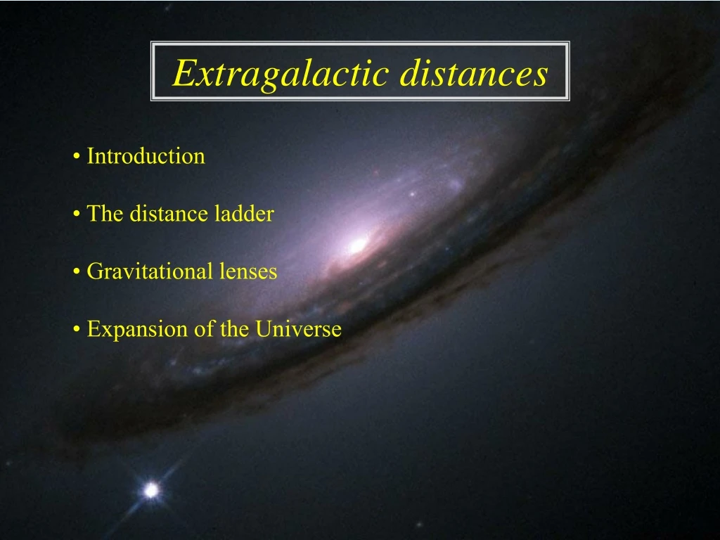
Extragalactic distances • Introduction • The distance ladder • Gravitational lenses • Expansion of the Universe
Introduction Since the beginning of 20th Century, there were a number of fundamental scientific discoveries in the study of the Universe Now we know that: • There was a beginning (Big Bang) a few billion years ago • Since then, the Universe is in expansion • Nuclear reactions in the very hot `post Big Bang´ era created the majority of the matter content of the Universe (H and He) Models of evolving Universes
Introduction - 2 • When matter became transparent (T ~ 3000 K), photons `decoupled´ from matter and began to propagate freely • Their wavelengths increased with the expansion of space, bringing them into the microwave domain: they constitute the cosmic microwave background (CMB) • The CMB, discovered in 1964 by Penzias and Wilson, is one of the best confirmations of the Big Bang model • Recent experiments measured with high accuracy the CMB spectrum • COBE satellite (1987 – 1993) → TCMB = 2.725 ± 0.002 CMB spectrum
Introduction - 3 • The satellites WMAP, launched in 2001, and Planck, launched in 2009, measured with high accuracy the CMB anisotropies. These tiny fluctuations (ΔT/T ~ 10−5) allow to determine the cosmological parameters CMB fluctuations (Planck mission)
Introduction - 4 • The analysis of WMAP data brought us in the precision cosmology era • The `standard cosmological model´, accepted by the majority of specialists, had the following parameters (after 9 years of data) : – total density (supposed = 1) Ω0 = 1.0 (1.02 ± 0.02) – baryonic matter density: Ωb,0 = 0.0463 ± 0.0024 – total matter density: Ωm,0 = 0.279 ± 0.023 – cosmological constant: ΩΛ,0 = 0.721 ± 0.025 – Hubble constant: h0 = 0.700 ± 0.022 (convention: H0 = 100 h0 km/s/Mpc) – age of the Universe (Gyr): t0 = 13.74 ± 0.11
Introduction - 5 • The analysis of Planck data has further increased the precision of the results • The new `standard cosmological model´, accepted by the majority of specialists, now has the following parameters: – total density (supposed = 1) Ω0 = 1.0 – baryonic matter density: Ωb,0 = 0.0486 ± 0.0014 – total matter density: Ωm,0 = 0.314 ± 0.020 – cosmological constant: ΩΛ,0 = 0.686 ± 0.020 – Hubble constant: h0 = 0.674 ± 0.014 (convention: H0 = 100 h0 km/s/Mpc) – age of the Universe (Gyr): t0 = 13.813 ± 0.058
Introduction - 6 All is best in the best of worlds… → What more to say? THE END…
• + degeneracy between Ω0 and h0 Ω0 Ωb,0 Ωd,0 ΩΛ,0 h0 1.00 0.046 0.22 0.73 0.72 1.05 0.081 0.39 0.58 0.55 1.10 0.111 0.54 0.45 0.45 1.20 0.171 0.83 0.20 0.37 Power spectrum of the fluctuations Introduction - 6 All is best in the best of worlds… … if one does not look too close, as: • the WMAP/Planck results are obtained by adjusting a model of fluctuations at the time of decoupling onto the observations → how far can we trust the model?
• observational: determine h0 → distance scale Ω0 Ωb,0 Ωd,0 ΩΛ,0 h0 1.00 0.046 0.22 0.73 0.72 1.05 0.081 0.39 0.58 0.55 1.10 0.111 0.54 0.45 0.45 1.20 0.171 0.83 0.20 0.37 Introduction - 7 The different models listed in the table reproduce the measured CMB fluctuations → one must fix Ω0 or h0 in another way: • philosophical: if Ω0 ≈ 1 then Ω0 = 1 Power spectrum of the fluctuations
The distance scale Measurement of distances: One of the most difficult problems in modern astrophysics! → proceed by steps From nearest objects… … to most distant ones → cosmological distance scale Danger: propagation of errors Georgia O’Keeffe « Ladder to the Moon »
The distance scale - 2 The parallax The distance to relatively nearby stars can be obtained by measuring their annual parallax The most accurate parallaxes have been measured by the Hipparcos satellite (HIgh Precision PARallax COllecting Satellite) of ESA, launched in 1989 The accuracy is ~0.001 arcseconds → distances to stars at 100 pc are known with a ~10% accuracy NB: 1 pc = 206265 AU = 3.26 LY The Hipparcos satellite
The distance scale - 3 Distance modulus Apparent magnitude: m = magnitude of the observed object, at its actual distance d Absolute magnitude: M = magnitude the object would have at a distance of 10 parsecs m = −2.5 log Fd + C Fd = L / 4πd2 M = −2.5 log F10 + C F10 = L / 4π102 Distance modulus: (d in parsecs) δm = m− M = −5 + 5 log d Distance measurement commonly used in astrophysics Must be corrected for dust absorption if present
The distance scale - 4 Cepheids 1912: Henrietta Leavitt finds that the period of Cepheids is a function (~proportional) of their luminosity These stars are luminous → observable at rather large distances → very useful distance standards (standard candles) Difficulties: • The distance to some Cepheids must be known to calibrate the relation • The period – luminosity relation depends on the star’s chemical composition
The distance scale - 5 Distances to galactic Cepheids – parallaxes Accurate parallaxes measured by HST Benedict et al. 2007 AJ 133, 1810: (10 galactic Cepheids) → adjustment of a straight line: MX = a + b (log P − 1) (P in days) X corresponds to the adopted index: V, I, K or WVI = V− 2.52 (V −I) (color correction to take into account the finite width of the Cepheid instability strip)
The distance scale - 6 Calibration of Cepheids vrad (spectro) → ΔR + Δθ (interfe-rometry) → d
The distance scale - 7 Calibration of LMC Cepheids Hundreds of Cepheids discovered by the OGLE program in the Large Magellanic Cloud (LMC) → largest and most precise sample available MW = a + b (log P − 1) With W = V − 2.45 (V −I) Is there a dependency on metallicity Z? (ZLMC < ZGal) On the basis of all available data, the opinion is divided…
The distance scale - 8 Distance to the Large Magellanic Cloud Importance of LMC for calibrating distances → determine its distance → many methods used, e.g.: • eclipsing binaries (ex.): 45.7 kpc (± 3%) • comparison of galactic and LMC cepheids: 47.9 kpc (± 2%) • luminous echoes reflected by the ring around SN1987a: 51.8 kpc (± 6%) Uncertainty > 10% remains… + take into account thickness and inclination of the LMC(non negligible)
The distance scale - 9 Uncertainties in the Cepheid distances • Calibration: ~ 10 % • Metallicity: ??? – is its effect significant? – in case it is, determination of metallicity: can not be done for the Cepheid but only for its galaxy → uniformity of metallicity in the galaxy? (very dubious for spirals) • Absorption by dust→ requires measurement of reddening – less important in IR (but Cepheids less bright in IR) – is often the main source of uncertainty
The distance scale - 10 Type Ia Supernovae (SNIa) To go further than Cepheids: we need brighter objects • Transfer of matter on a white dwarf in a binary system → Nova eruptions and progressive accumulation of matter • When M > 1.4 M → explosion of the star → Lmax≈ constant MB≈ MV≈ –19.3 at max brightness • mobs must be corrected for reddening by dust → possible by observing through several filters and comparing with `standard´ colors • also allows the `k-correction´
Light curves of nearby SNIa Corrected light curves The distance scale - 11 Type Ia Supernovae • Problem: in the 1990s, it was found that not all SNIa have the same maximum luminosity → would not be as good standard candles as thought! • By studying nearby SNIa, one notices a correlation between maximumluminosity and the rate of decrease in the post-maximum light curve → allows to calculate Lmaxfrom the shape of the light curve (stretch method)
The distance scale - 12 Type Ia Supernovae • SNIa are ~13.3 magnitudes brighter than the brightest Cepheids → allow to reach distances 500 times larger (with present instruments, more than 1000 Mpc) • SN explosions are rare phenomena → require to observe a large number of galaxies → ambitious observing programmes since the 1990s: – Supernova Cosmology Project – High-Z Supernova Search
m m mlim log(distance) log(distance) The distance scale - 13 The Malmquist bias • In a magnitude-limited sample (thus not volume-limited) • with a dispersion σ (intrinsic or observational) • the more distant are the objects (thus apparently fainter), the stronger the tendency to bias towards the brightest → most distant objects kept in the sample appear too bright on average → that bias must be corrected, it requires to know σ(distance)
The distance scale - 14 Secondary distance indicators • Contrary to primary indicators, they need to be calibrated from galaxies whose distances are known • which is, in fact, partially the case of Cepheids, which depend on the distance to the LMC • and thus also of SNIa, which are calibrated by determining the distance of their host galaxies from Cepheids • calibration done for the nearby SNIa, the more distants being assumed to have the same properties (no evolution with the age of the Universe) → distinction a bit fuzzy between primary and secondary indicators
The distance scale - 15 Magnitude at the tip of the giant branch • The tip of the giant branch of the most metal-poor globular clusters [Fe/H] ~ −1.5 reaches the same MV~ −2.5 • even smaller dispersion in MI≈ −4.05 ± 0.02 • distance of galactic globular clusters given by RR Lyrae stars → independent of Cepheids (but similar method)
The distance scale - 16 Luminosity function of globular clusters • φ(M)dM = number of clusters in the magnitude interval [M, M+dM] • φ(M) is well fitted by a gaussian function • the top (turnover) corresponds to the most numerous clusters • it seems to correspond to a `universal´ MB,0≈ −6.5 • distance estimated by measuring mB,0 • works best for galaxies with many clusters • calibration on the Virgo cluster → depends on this cluster distance
The distance scale - 17 Planetary nebulae luminosity function (PNLF) • Number of planetary nebulae (PN) in a galaxy (or a group/cluster) as a function of their luminosity in the forbidden line of oxygen 2 times ionized [O III] at 500.7 nm (NB: PN spectrum = emission lines – negligible continuum) • that line is very strong and allows to observe PN up to ~20 Mpc • there seems to be a cutoff (maximum luminosity) corresponding to absolute magnitude M5007≈ −4.53
The distance scale - 18 Planetary nebulae luminosity function (2) • Comparison of distances obtained by the PNLF and by the Cepheid methods → precision of the PNLF method estimated by the dispersion σ of the points around the straight line (M31 sets the zero point) → one obtains σ ≈ 8% (internal precision, does not take systematic errors into account)
The distance scale - 19 Brightness fluctuations • The more distant a galaxy is, the more stars fall on average on a single pixel of the CCD → the more the galaxy appears `smooth´ (less granular) on the images • Poisson statistics: σ(N) = N1/2→ σ(N)/N = N−1/2 → relative fluctuations decrease when N increases ↔d increases • Best adapted to elliptical galaxies (because they contain only stars) • With the resolution of HST, that method can reach ~ 100 Mpc
The distance scale - 20 The Tully-Fisher relation • Relation between luminosity of a spiral galaxy and its maximum rotation velocity • More precise in the IR as less influenced by dust and star formation regions → better represents the global mass • σ(near-IR) ≈ 40% (can go down to 10% for carefully selected galaxies) • Applied to Virgo and Coma clusters → 3D maps of these clusters • Allows to reach distances > 100 Mpc
The distance scale - 21 Relation D-σ • Relation between effective diameter D and velocity dispersion σ in bright elliptical galaxies • No Cepheids to calibrate the method in these galaxies → relative distances between clusters: Cluster 1: log D1 = a log σ + C1 Cluster 2: log D2 = a log σ + C2 Surface brightness independent of d → • Lower dispersion in IR • Very bright galaxies → allows to reach large distances
The distance scale - 22 Comparison of distances for the Virgo cluster → d ~ 16 Mpc
Gravitational mirages • The distance scale (cosmological distance ladder) is built step by step • The most distant indicators (ex: SNIa) are `locally´ calibrated from indicators in lower steps (ex: Cepheids) • This method is very sensitive to error propagation: any error on a step will propagate to upper steps • Ex: the ~10% uncertainty in the Cepheids calibration (that depends in large part on the distance of the LMC) will propagate to SNIa → it is desirable to have another method for measuring distances that would be independent of this `standard´ distance ladder
Gravitational mirages - 2 Atmospheric mirages Our brain interprets vision by assuming light propagates on straight lines If the refraction index varies → light rays are deflected → we `see´ the object in another direction → possibility of several images – possibly • deformed • reversed
Gravitational mirages - 3 Gravitational mirages General relativity → space-time curvature → light rays are deflected in the vicinity of a mass concentration → possibility of several images – possibly • deformed • magnified → gravitationalmirage by analogy with atmospheric mirage • the object that deflects light is called gravitational lens • effect predicted by Einstein who thought it would be unobservable as only stars were known at his time as lens candidates • predicted by Zwicky in the 1930s with galaxies as lenses
Gravitational mirages - 4 The first gravitational mirage 1979: Walsh, Carswell and Weymann were studying quasar spectra They realized that 2 quasars separated by 6″ have the same spectrum → hypothesis: these are two images of the same quasar – confirmed by the detection of the lens galaxy, close to one image Quasars are good candidates: very luminous → observable far away → higher probability to have a galaxy in front of them HST The 2 images of quasar Q0957+561
Gravitational mirages - 5 Mirages and distances • Refsdal, 1964: different optical paths have different lengths + gravitational time dilation → time delay between the detection of an event in different images If the quasar varies, one can measure this delay If the mass distribution is known: → one obtains a distance Δd = cΔt → cosmological distance
Theory of gravitational mirages • General relativity predicts that a light ray passing at a minimal distance ξ from a point-like object of mass M is deflected by an angle: • Simplifying hypotheses: (1) The whole deflecting mass is at the same distance Dd from the observer (thin lens) → observer plane, deflector plane, source plane → distances Dd , Ds ,Dds If curved space: Ds≠ Dd + Dds
Theory of gravitational mirages - 2 (2) All the angles considered are small → (distances are angulardiameterdistances − cf. cosmology chapter) • β = angle between deflector and actual position of the source • θ = angle between deflector and apparent position of the source • α = reduced deflection angle = apparent angular displacement of the source from S to S’ → β = θ− α(θ) (3) • one also has:
Theory of gravitational mirages - 3 General lenses • If lens not point-like → one adds the deflections of the ≠ point masses where is the surface mass density at point • Cylindrically symmetrical lens (circular in the lens plane): → → where is the mass in the disk of radius ξ around the center
Theory of gravitational mirages - 4 Einstein ring By introducing (1) or (5) in (4), we get: But ξ = θ Dd→ Introducing (6) in (3): If the source is exactly behind the lens (β = 0): → circular symmetry → ring of radius θE If the distances are known → the mass of the lens inside the Einstein radius can be determined
Theory of gravitational mirages - 5 Critical density Mean surface density inside the angular radiusθ: = critical density (9) κ = density measured in units of the critical density = convergence If κ > 1 (Σ > Σcr) → formation of multiple images
Theory of gravitational mirages - 6 Image positions Point-like deflector: quadratic equation → 2 solutions: (11) For a point-like deflector, always two images, one inside and the other outside the Einstein ring If β >> θE→ θ+ = β(no deflection) and θ− = 0 (but see below)
Theory of gravitational mirages - 7 Image magnification Surface brightness is unchanged (no absorption nor emission of photons) → magnification μ= ratio surface image / surface source [at one dimension: if x is imaged according to y = y(x), a small interval Δx will be imaged as Δy, with Δy ≈ (dy/dx) Δx the jacobian (12) generalizes this in two dimensions] Valid for `small sources´
Theory of gravitational mirages - 8 Image magnification Lens with circular symmetry Using equation (11) and defining u as the separation image-lens in units of the Einstein radius: u = β / θE one gets: • image + is always magnified • image − can be magnified or demagnified, according to u • if the source is inside the Einstein ring, μ > 1.34
Theory of gravitational mirages - 9 Total magnification • if u → 0, μ→ ∞ (only for a point source) • if u → ∞, μ→ 1 In cases where the image separation is too small to be resolved by existing instruments (typically for too small deflector masses), the total magnification can nonetheless be measured
Types of gravitational mirages • In cases with multiple images (strong lensing), the typical separation between the different images is given by: • In this case, we have → θE thus gives the characteristic image separation • If lens = Milky Way star: (in arcseconds) → image separation is typically 1/1000 arcseconds → not observable with present-day telescopes → Einstein’s conclusion on non-observability of mirages
Types of gravitational mirages - 2 Micro and macrolensing • If lens = external galaxy (z ~ 0.5) and source = quasar (z ~ 2): (in arcseconds) (macrolensing: one can observe several images) • If lens = star in the deflecting galaxy and source = same quasar: → θE ~ 10−6 arcseconds (microlensing: one can only observe total magnification)
Types of gravitational mirages - 3 Critical curves and caustics • Image magnification is given by (12): • Regions in the lens plane where the determinant cancels correspond to an infinite magnification (for a point source): they are called critical curves • Projections of these critical curves on the source plane are called caustics • For circularly symmetrical lenses, critical cuves are circles • For point lenses, they reduce to a point • If the source is extended, magnification cannot be infinite
cusp fold Types of gravitational mirages - 4 Critical curves and caustics • Figure below illustrates the critical curves (left) and caustics (right) for an elliptical lens • Non symmetrical lenses (like this one) can give rise to more than two images • Numbers indicate regions of the source plane giving rise to 1, 3 or 5 images • In the 3 or 5 image cases, one of them is strongly demagnified → one observes only 2 or 4 images
Types of gravitational mirages - 5 Image configurations As a function of: • mass distribution in the lens • alignment source – lens – observer one can observe differents image configurations: • doubles • quadruples • arcs • ring Only extended sources give rise to arcs or rings