Download

1 / 48
480 likes | 617 Vues
This talk by Amy Barger delves into the significant advancements in distant Active Galactic Nuclei (AGN) studies enabled by Chandra and XMM X-ray surveys. It highlights the ability to map AGN history through hard X-ray surveys and the critical need for spectroscopic identifications versus photometric redshifts to construct accurate luminosity functions. Barger discusses the challenges in source classification and uncertainties in the X-ray background measurement while exploring the insights gained from comparing X-ray and optical selected AGN samples.

E N D
Extragalactic Surveys Amy Barger
Where Are We? Chandra/XMM have revolutionized distant AGN studies Now possible • to map the history of a large fraction of the AGN population using hard X-ray surveys, and • for the first time, to compare high-redshift & low-redshift samples chosen in the same rest-frame hard energy (2-8 keV) band
Striking how modest the number of X-ray sources is compared to the number of optical sources
What Do We Need to Map the AGN History? Pyramid of surveys running from large area, shallow surveys to CDF-N level ultradeep surveys [that is, as large a base as possible and as high a tip as possible] One of the key issues: can we justify needing even deeper fields, say up to 5 Ms? For example, to measure the faint end of the luminosity function in the z=2-3 range?
AGN Steffen et al. 2004
What Else Do We Need? Spectroscopic identifications! Photometric redshifts are a possible substitute---with the addition of NIR and MIR data, we are able to make reasonable photometric redshift estimates and use them to construct luminosity functions • However, they do not tell about the spectral type of the galaxy producing the X-ray light, and . . .
. . . there is danger in the scatter: if a phot-z scatters a source into a region where there are not many objects (say, a catastrophic error scattering a low-z source to z~3), then one can get the LF there very wrong GOAL: have the spectroscopic identifications be as complete as possible (wide-field NIR spectrographs should help for z=1.6-2.6) Lrf(2-8 keV)=1044 ergs/s 1043 ergs/s Red=spec-zs Purple=phot-zs Diamonds=unid Negative values mean nuclear dominated
Additional Needs Really important to have complete wavelength coverage to understand the spectral energy distributions of the AGN Also want to know if there are other AGN sufficiently thick that they are not being seen in current hard X-ray surveys
Above f(2-8 keV)~10-14 ergs cm-2 s-1, 80-90% of hard X-ray sources have redshifts, while below this flux, ~60% ASCA CDF-N CLASXS CDF-S Barger et al. 2005
All All z HEX BLAGN What Do We Mostly Agree On?
The Good News There is an astonishing amount of agreement---we understand the X-ray samples very well! But there still are issues that need to be resolved
Uncertainties in the X-ray background measurement are still at the 10-20% level, so we cannot accurately determine the resolved fraction of the XRB. This is a tricky issue, particularly for population synthesis modelers who need to decide what additional component to add in. Hickox & Markevitch 2006
Source Classification One of the most important issues is that of source classification, and what we mean by the various classes Most groups use the four optical spectral classes of Szokoly et al. 2004, which are crude by the standards of optical AGN specialists: absorbers, star formers, high-excitation sources (HEX), broad-line AGN (BLAGN; FWHM>2000 km/s)
Relative Contributions to 2-8 keV Light by Spectral Class All All z HEX BLAGN 33% BLAGN 7% HEX 27% (“XBONG”; >1042 ergs/s) 3% (“OBXF”; <1042 ergs/s) 30% Unidentified Can now look at the X-ray colors by optical spectral class
BLAGN are nearly all soft and show essentially no visible absorption in X-rays, consistent w/our understanding of them as unobscured 2 x 1021 cm-2 Barger et al. 2005
All the other AGN are well-described by a power-law spectrum with photoelectric absorption spread over a wide range of NH 3 x 1022 cm-2 Open squares---absorbers and star formers Solid squares---high-excitation signatures Triangles---unidentified sources Barger et al. 2005
X-ray Luminosity Functions When computing rest-frame hard (2-8 keV) X-ray luminosity functions, one of the interesting things is to make a comparison with optically-selected QSO samples To do that, one needs to use the optical spectroscopic classifications to determine the BLAGN luminosity function separately
ALL Z=0,0.4,0.8 shells BLAGNs LOCAL (RXTE) Sazonov & Revnivtsev (2004) As move to higher z, all the sources are increasing in L while the LFs are maintaining the same shapes; if drift the x-axis, plots look very much the same from z=0 to z=1.2 Barger et al. 2005
The Steffen Effect BLAGN dominate the number densities at the higher X-ray luminosities This therefore says that almost all luminous objects are unobscured, which instantly says there must be some luminosity dependence on the obscuration, since we know there is a substantial fraction of obscured sources at the lower luminosities Z=0,0.4,0.8 shells BLAGN
The shape of the BLAGN relative to the shape of the total stays pretty much the same with z, since both are obeying PLE This says that the BLAGN fraction---that is, the ratio of the integrals---stays the same over interval z=0-1.2 However, the objects that are BLAGN are much less luminous at low-z than at high-z Z=0,0.4,0.8 shells
Open Question This is a rather bizarre situation! What is it that leaves certain properties, such as the relative shapes of the two luminosity functions, so invariant, while changing the luminosities so much? In other words, why should a lower luminosity source be a BLAGN at lower redshifts, but a similar luminosity source not be a BLAGN at z=1?
Higher Redshift Intervals Incompleteness larger here, but phot-zs indicate unids mostly lie in z=1.5-3 interval Shapes no longer well-represented by the maximum likelihood fits to the z=0-1.2 HXLFs computed at z=1 (blue curves): Thus, PLE does not continue beyond z=1.2 There are fewer low-L sources than one expects, and so the light density is more dominated by higher L sources at these redshifts
Good agreement between the optical and X-ray selected LFs! Our optical spectroscopic classification of BLAGN is consistent with that of groups doing direct optical selection Richards et al. 2005
Classification Issue Up to now, we have just considered the optical spectral properties of the X-ray sources, but it is very reasonable to try to go the other way and ask, ‘‘Just by looking at the X-ray properties, is it possible to tell whether a source is what an optical AGN specialist would call a BLAGN?“
No, this is not so clear-cut. Have we optically misclassified some sources w/soft X-ray spectra? 3 x 1022 cm-2 Open squares---absorbers and star formers Solid squares---high-excitation signatures Triangles---unidentified sources Barger et al. 2005
HEX sources are quite easily distinguished from BLAGN and from the low excitation sources weak Hb narrow CIV Noise is dominated by the noisiest spectrum Cowie & Barger
The low excitation sources have strong Hb and do not show signs of NeV or of broad underlying Balmer lines. 68 of the sources show no emission lines at all strong Hb Noise is dominated by the noisiest spectrum Cowie & Barger
Are BLAGN Being Lost in Other Ways? Are selection effects (e.g., galaxy dilution or spectral selection effects, such as whether spectrum includes Ha) causing one to misclassify BLAGN at low X-ray luminosities? [Moran et al. 2002; Silverman et al. 2005; Heckman et al. 2005] For example: could the absence of BLAGN at low X-ray luminosities be explained if the nuclear UV/optical light were being swamped by the host galaxy light?
Absorption line (in some cases, don’t see any UV nuclei) z Starbursts LINERs & Seyfert 1s Seyfert 2s ACS GOODS BLAGN
Well-known that the nuclear UV magnitudes and the X-ray fluxes for BLAGN are strongly correlated • If galaxy dilution hypothesis were correct, would expect the non-BLAGN to be similarly correlated when we isolate their nuclear UV/optical light
Instead, turns out that, in general, the nuclei of the non-BLAGN are much weaker relative to their X-ray light than the BLAGN Negative values mean nuclear dominated
Thus, absence of BLAGN at low X-ray luminosities is not a dilution effect In general, non-BLAGN really have weaker UV/optical nuclei relative to the X-rays Thus, we are left with the situation that there is not a one-to-one correspondence---we cannot select only optical BLAGN just by looking at the X-ray properties
G. Hasinger SlideOptically Identified Hard Samples type-1: optical BLAGN, or galaxy with LX>42, HR<-0.2 type-2: optical NLAGN, or galaxy with LX>42, HR>-0.2
But then things get really confused! Sources with soft X-ray spectra are -mostly BLAGN at high X-ray luminosities -HEX sources become a significant fraction at intermediate Ls -we do not see AGN signatures in the optical spectra at low Ls
Conclude: if one is going to split X-ray luminosity functions by class, one should do it based on optical spectral class alone or by X-ray color alone, but one should not try to mix them, because we do not understand how to relate one to the other But, maybe it would make sense just to split X-ray luminosity functions based on the X-ray colors alone, since that may be the best measure of whether a source is obscured or not
An X-ray color cut with G=1.2 basically reproduces the BLAGN LF at high Ls but adds in sources at faint Ls, flattening out the LF, but it is a little sensitive to where you place the cut---a higher gamma cut makes it look much more like the BLAGN LF. The Steffen Effect still holds, however. All z=0.5-1 G=1.2 BLAGN
2-8 keV comoving energy density production rate drops rapidly from z=1 to z=0; peak is in interval z=0.8-1.2 Open=spectroscopic sources Solid=all, including phot-zs; no ids put at z=3 Negative values mean nuclear dominated At z<1.2, only 1/3 is due to broad-line AGNs
Cumulative growth of AGNs from Chandra (red curve) compared with the cumulative SFH Although both form most of their mass at late times (z~1), the AGN growth shows a slightly different history & is running later than the SFH; if AGN feedback has a significant effect, the relative histories can help diagnose that. Would like deeper images to check whether there is a fainter z=5-6 X-ray population. Potential hidden gottcha: presence of Compton-thick AGN.
What Might We Be Missing? • Deep MIR and radio images are an obvious avenue for searching for highly-obscured AGNs, since extinction in the MIR & radio is small • People have tried to use combined MIR & radio selections, but to obtain a reliable upper limit on the possible population of X-ray undetected, obscured AGNs, a clean selection is needed • Here we use a pure microJansky radio survey selection in the HDF-N field • (207 sources to 40 mJy in a 310 arcmin2 area)
The well-known correlation between radio power & FIR luminosity makes it possible to estimate the total FIR luminosity of a galaxy from its radio power (this correlation has been empirically determined for both star formers & radio-quiet AGNs) • Even with Spitzer, this is still the most robust way • limited MIPS sensitivities at 70 and 160 mm
-the conversion from 24 mm to total FIR luminosity depends strongly on the template spectral energy distributions used to K-correct the data Barger et al. 2007 (astro-ph/0609374)
What fraction of the X-ray light is coming from the different X-ray and radio populations?
It is sufficient for us to measure the X-ray surface brightnesses from known X-ray sources in the CDF-N & see that they are roughly consistent with the HEAO1/A2 XRB (Revnivtsev et al. 2005) Z=0,0.4,0.8 shells Barger et al. 2007
X-ray sources that are not radio sources and the total radio sample each contribute 50% of the X-ray light at 4-8 keV, but most of the radio sample contribution is from X-ray luminous radio sources Z=0,0.4,0.8 shells Total radio X-ray sources that are not radio Barger et al. 2007
Contributions from the remaining radio sources are very small Z=0,0.4,0.8 shells Radio sample without X-ray luminous counterparts (2.3% at 4-8 keV) Radio sample without any X-ray counterparts (1.2% at 4-8 keV) Barger et al. 2007
Thus, the current radio source population cannot account for the background light that has been suggested may be missing at 4-8 keV Indeed, the percentages are about a factor of 5 lower than those predicted for 1024 cm-2 sources at these energies in typical XRB synthesis models (e.g., Gilli, Comastri, Hasinger 2006)
Summary • X-ray data are consistent with many of the non-BLAGN (the dominant population) having high column densities • AGN evolve very rapidly to z~1.2, consistent with pure luminosity evolution to that redshift • z~1 is where the bulk of the supermassive black hole population forms • Simple unified model is not correct, whether one uses X-ray color or optical spectral classification---there are far fewer low X-ray luminosity, unobscured sources than obscured • Contributions to the 4-8 keV light from the X-ray faint radio population is very small, and hence these sources are unlikely to contribute substantially to the XRB at even higher energies