Nonlinear Time Series Classification Using Reconstructed Phase Space for Phoneme Recognition
110 likes | 216 Vues
This paper introduces a novel approach for phoneme recognition using nonlinear modeling techniques based on reconstructed phase space. It explores nonlinear classifiers, clustering methods, and frequency-based techniques to classify speech signals accurately. The algorithm involves steps like data analysis, Gaussian Mixture Models (GMMs) for signal trajectory densities, and Bayesian classifiers for differentiation. Experimentation on the TIMIT speech corpus demonstrates the approach's effectiveness, highlighting the challenges of insufficient training data. References include key works in time series classification and nonlinear dynamics.

Nonlinear Time Series Classification Using Reconstructed Phase Space for Phoneme Recognition
E N D
Presentation Transcript
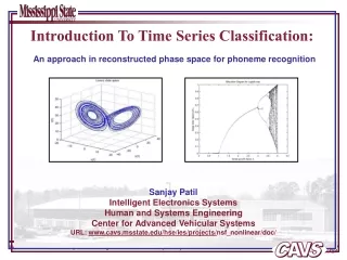
Introduction To Time Series Classification: An approach in reconstructed phase space for phoneme recognition Sanjay Patil Intelligent Electronics Systems Human and Systems Engineering Center for Advanced Vehicular Systems URL: www.cavs.msstate.edu/hse/ies/projects/nsf_nonlinear/doc/
Abstract • Present nonlinear classifiers: • clustering and similarity measurement techniques, eg. NN, SVM. • Existing time-domain approaches: • a priori learned underlying pattern of template base. • Frequency-based techniques: • spectral patterns based on first and second order characteristics of the system. • Current work (as described in the paper): • modeling of signals in the reconstructed phase space.
Slightly different notations than usually used by other researchers. • Motivation (why did I read it?) An attempt to find an approach to model the speech signal using nonlinear modeling technique. • Takens and Sauer – new signal classification algorithm. • Time series of observations sampled from a single state variable of a system • Reconstructed space equivalent to the original system
The Approach • Two methods to tackle the issue: • Build global vector reconstructions and differentiate signals in a coefficient space. [Kadtke, 1995] • Build GMMs of signal trajectory densities in an RPS and differentiate between signals using Bayesian classifiers. [Authors, 2004] • The steps (Algorithm): • Data Analysis – normalizing the signals, estimating the time lag and dimension of the RPS. • Learning GMMs for each signal class – deciding the number of Gaussian mixtures, parameters learning by Expectation-Maximization (EM) algorithm. • Classification – going through the above steps for the SUT (signal under test), using Bayesian maximum likelihood classifiers
Algorithm in details and Issues • Data Analysis – • normalizing the signals • Each signal is normalized to zero mean and unit standard deviation. • estimating the time lag • Using first minimum of the automutual information function. • Overall time lag is the mode of the histogram of the first minima for all signals. • estimating dimension d of the RPS • Using global false nearest-neighbor technique. • Overall RPS dimension is the mean plus two standard deviations of the distribution of individual signal RPS dimensions. • How do you normalize the signal to zero mean and unit standard deviation? • What is automutual information function? • How do you implement the global false nearest-neighbor technique?
Algorithm in details and Issues • 2. Gaussian Mixture Models – • Insert all the signals for a particular class into the RPS for a particular d and selected in previous step, • GMM: • Where, M = # of mixtures, • N(x;, ) = normal distribution with mean and covariance matrix • W = mixture weight with the constraint • GMMs estimated using Expectation-Maximization (EM) algorithm. • How is EM algorithm implemented? • Classification accuracy depends on M, So how to determine the value of M? • What is value of M determined from the underlying distribution of the RPS density?
Algorithm in details and Issues • 3. Classification – • Maximum Likelihood estimates from previous step are: • Where, mean , covariance matrix , mixture weight W • Using Bayesian maximum likelihood classifiers: • Compute the conditional likelihoods of the signal under each learned model • Select the model with highest likelihood. • How are the conditional likelihoods computed?
Experiment details and Issues • TIMIT speech corpus: • 417 phonemes for speaker MJDE0. • 6 spoken only once, 47 classes in total (out of the standard 48 classes) • Sampling frequency 16KHz, Signal length – 227 to 5,201 samples • Phoneme boundaries and class labels determined by a group of experts • 25 iterations of EM algorithm are used. • Classification accuracy is around 50% (50% for 16GMMs, @48% for 32GMMs) [reason – due to insufficient training data] • Approach is compared with time delay NN with nonlinear one step predictor and minimum prediction error classifier. • Details on how the testing is done is missing. • How is insufficient training data causing reduction in accuracy for increase in GM mixtures?
References • R. Povinelli, M. Johnson, A. Lindgren, and J. Ye, “Time Series Classification using Gaussian Mixture Models of Reconstructed Phase Spaces,” IEEE Transactions on Knowledge and Data Engineering, Vol 16, no 6, June 2004, pp. 770-783. (the referred paper) • F. Takens, “Detecting Strange Attractors in Turbulence,” Proceedings Dynamical Systems and Turbulence, 1980, pp 366-381. (background theory) • T. Sauer, J. Yorke, and M. Casdagli, “Embedology,” JournalStatistical Physics, vol 65, 1991, pp 579-616. (background theory) • A. Petry, D. Augusto, and C. Barone, “Speaker Identification using Nonlinear Dynamical Features,” Choas, Solitions, and Fractals, vol 13, 2002, pp 221-231. (speech related dynamical system) • H. Boshoff, and M. Grotepass, “The fractal dimension of fricative Speech Sounds,” Proceddings South African Symposium Communication and Signal Processing, 1991, pp 12-61. (speech related dynamical system) • D. Sciamarella and G. Mindlin, “Topological Structure of Chaotic Flows from Human Speech Chaotic Data,” Physical Review Letters, vol. 82, 1999, pp 1450. (speech related dynamical system) • T. Moon, “The Expectation-Maximization algorithm,” IEEE Signal Processing Magazine, 1996, pp 47-59. (expectation-maximization algorithm details) • Q. Ding, Z. Zhuang, L. Zhu, and Q. Zhang, “Application of the Chaos, Fractal, and Wavelet Theories to the Feature Extraction of Passive Acoustic Signal,” Acta Acustica, vol 24, 1999, pp 197-203. (frequency based speech dynamical system analysis) • J. Garofolo, L. Lamel, W. Fisher, J. Fiscus, D. Pallet, N. Dahlgren, and V. Zue, “TIMIT Acoustic-Phonetic Continuous Speech Corpus,” Linguistic Data Consortium, 1993. (speech data set used for experiments)