Time Series Analysis
Time Series Analysis. What is Time Series Analysis? The analysis of data organized across units of time. Time series is a basic research design Data for one or more variables is collected for many observations at different time periods Usually regularly spaced May be either

Time Series Analysis
E N D
Presentation Transcript
Time Series Analysis • What is Time Series Analysis? • The analysis of data organized across units of time. • Time series is a basic research design • Data for one or more variables is collected for many observations at different time periods • Usually regularly spaced • May be either • univariate - one variable description • multivariate - causal explanation
Time Series vs. Cross Sectional Designs • It is usually contrasted to cross-sectional designs where the data is organized across a number of similar units • The data is collected at the same time for every observation • Thus: • A data set consisting of 50 states for the year 1998 is a cross-sectional design. • A data set consisting of data for Alabama for 1948 – 1998 is a time series design.
Why time series or cross sections? • Depends on your question • If you wish to explain why one state is different from another, use a cross-sectional design • If you wish to explain why a particular state has changed over time, use a time series design
Time-Series Cross-Sectional Designs • There are techniques for combining the two designs. • Due to concerns for autocorrelation, and estimation, we will examine this design later in the course
Conceptual reasons to consider time series models • Classic regression models assume that all causation is instantaneous. This is clearly suspect. • In addition, behaviors are dynamic - they evolve over time.
What is Time anyway? • Time may be a surrogate measure for other processes (i.e. maturation, aging, growth, inflation, etc.) • Many of the processes we are interested in are described in terms of their temporal behavior (Arms races, growth and decay models, compound interest) • Statistical tools may often improve their degrees of freedom by using time series methods. (Sometimes this means larger n)
Why time series? • My personal view is that Time Series models are theoretically fundamentally more important than cross-sectional models. • The models that we are really interested are those that help us model how systems change across time - vis a vis what they look like at any given snapshot in time.
The Nature of Time Series Problems • Please note: Time series problems are theoretical one - they are not simply statistical artifacts. When you have a time series problem, it means some non-random process out there has not been accounted for.
A Basic Vocabulary for Time Series • Period • Cycle • Season • Stationarity • Trend
Periodicity • The Period • A Time series design is simple to distinguish because of its period. The data set is comprised of measures taken at differing points in time. The unit of the analysis is the period. (i.e. daily, weekly, monthly, quarterly, annual, etc.) • Note that the period defines the discrete time intervals where data measurement is taken
Cycle • Uses classic trigonometric functions such as the sine and cosine to examine periodicity in the data. • This is the basis for Fourier Series and Spectral Analysis. • Used primarily in economics where they have data series measured over a long period of time with multiple regularly occurring and overlapping cycles. (Rarely used in Political Science, but try the commodity markets, with hog/beef/chicken cycles)
Cycles (cont.) • A simple cyclic or trigonometric function might look like this:
Cycles (cont.) • You could estimate a model like • But why would you? What theory do you have that suggests that political data follow such trigonometric periodicity?
Seasonality • Season • Sometimes, when a relationship or a data series has variation related to the unit of time, we often refer to this as seasonality. • (e.g Christmas sales, January tax revenues.) • This most often occurs when we have discrete data. • (Seasonality is thus the discrete data equivalent of the continuous data assumed by spectral analysis
Regression with Seasonal Effects • Estimating a regression model with seasonal behavior in the dependent variable is easy: • Where S1 is a seasonal dummy. • S1 is coded 1 when the observation occurs during that season, and 0 otherwise.)
Estimating Seasonality • Like all dummy variable models, at least one Season (Category) must be excluded from the estimation and the intercept represents the mean of the excluded season(s). • Failure to exclude one of the seasonal dummies will result in biased estimation at best and in all likelihood error messages about non-singular matrices or extreme multicolinearity. • The slope coefficients represent the change +/- from the intercept, and the t-tests are tests of whether the seasons are different from the intercept, not just different from 0.
Estimating Seasonality • Estimating regression models with seasonality is a popular and valuable method in many circumstances. • (i.e. estimating tax revenues)
Stationarity • If a time series is stationary it means that the data fluctuates about a mean or constant level. Many time series models assume equilibrium processes.
Non-Stationarity • Non-stationary data does not fluctuate about a mean. It may trend away or drift away from the mean
Trend • Trend indicates that the data increases or decreases regularly.
Drift • Drift means that the series ‘drifts’ away from its mean, but then drifts back at some later point.
Variance Stationaity • Variance Stationarity mans that the variation in the data about the mean (or trend line) is constant across time. • Non-stationary variance would have higher variation at one end of the series r the other.
A Basic Vocabulary for Time Series • Random Process/ Stochastic Process • The data is completely random. It has no temporal regularity at all.
A Basic Vocabulary for Time Series • Trend • Means that the data increases or decreases over time. • Simplest form of time series analysis • Uses a variable as a counter {Xi = 1, 2, 3, .. n} and regresses the variable of interest on the counter. • This gives an estimate of the periodic increase in the variable (i.e. the monthly increase in GNP • Problems occur for several reasons: • The first and last observations are the most statistically influential. • Very susceptible to problems of autocorrelation
Random- walk • If the data is generated by We call it a random-walk. • If B is non-zero, the data has a trend. • If B is equal to 0.0, then the series drifts away from the mean for periods of time, but comes back (hence often called drift, or drift non-stationarity)
Unit Root tests • A number of tests have emerged to test whether a data series is TSP or DSP. Among them, the Dickey-Fuller test. (More on this in a few weeks) • The current literature seems to suggest that regression on differences is safer than regression on levels, due to the implications of TSP and DSP. We will return to this later.
Autocorrelated error • Also known as serial correlation • Detected via: • The Durbin Watson statistic • The Ljung-Box Q statistic ( a 2 statistic) • Note that Maddala suggests that this statistic is inappropriate. • Probably not too bad in small sample, low order processes. • Q does not have as much power as LM test. • The Portmanteau test • Lagrangian Multiplier test
Autocorrelated error (Cont.) • If autocorrelation is present, then the standard errors are underestimated, often by quite a bit, especially if there is a trend present. • Test for AC, and if present, use • the Cochran-Orcutt method • the Hildreth-Lu method • Durbin’s method • Method of first differences • Generalized Least squares
Certain models are quite prone to • autocorrelation problems • Distributed Lags • The effect of X on Y occurs over a longer period, • There are a number of Distributed Lag Models • Finite distributed lags • Polynomial lags • Geometric Lags • Almon lag • Infinite Distributed Lags • Koyck scheme
Lagged Endogenous variables • In addition, there are models which describe behavior as a function of both independent influences as well as the previous level of Y. • These models are often quite difficult to deal with. • The Durbin-Watson D is ineffective - use Durbin’s h
Some common models with lagged endogenous variables • Naive expectations • The adaptive Expectations model • The partial adjustment model • Rational Expectations
Remedies for autocorrelation with lagged endogenous variables. • The 2SLSIV solution • regress Yt on all Xt’s, and Xt-1's. • Then take the Y-hats and use as an instrument for Lagged Y’s in the original model. • The Y-hats are guaranteed to have the autocorrelated component theoretically purged from the data series. • Have fun!
Non-linear estimation • Not all models are linear. • Models such as exponential growth are relatively tractable. • They can be estimated with OLS • But a model like is somewhat more difficult to deal with.
Nonlinear Estimation (cont.) • The (1-c) parameter may be estimated as a B, but the t-test will not tell us if c is different from 0.0, but rather whether 1-c is different from 0.0. • Thus the greater the rate of decay, the worse the test. • Hence we wish to estimate the equation in its intractable form. • There may be analytic solutions or derivatives that may be employed, but conceptually the grid search will suffice for us to see how non-linear estimation works.
The Backshift Operator • The backshift operator B refers to the previous value of a data series. • Thus • Note that this can extend over longer lags.
UNIVARIATE TIME SERIES • Autoregressive Processes • A simple Autoregressive modelThis is an AR(1) process. The level of a variable at time t is some proportion of its previous level at t-1. This is called exponential decay (if is less than unity - 1.0)
Autoregressive Processes • An autoregressive process is one in which the current value is a function of its previous value, plus some additional random error. • This is analogous to 1st order autocorrelation in regression analysis. • Keep in mind that with serial correlation we are talking about the residual, not a variable.
Higher Order AR Processes • Autoregressive Processes of higher order do exist: • AR(2), ... AR(p) • In general be suspicious of anything higher than a 3rd order process: • Why should life be so abstractly complex? Autoregressive Processes • The general form using Backshift notation is:
Moving average processes • Moving averages depend not on the level of the last time point, but rather on the last time point’s error. • Thus an MA(1) is represented by
The General MA(q) Process • The general MA(q) model is: • Again, higher order processes do exist MA(2), ... MA(q). • As with AR(p) processes, be suspicious of anything higher than a 3rd order process. • Why should life be so abstractly complex? • The general form using Backshift notation is:
ARIMA Models • Hence we have the following basic or frequently encountered models ARIMA(0,0,0) ARIMA(0,1,0) ARIMA(1,0,0) ARIMA(1,1,0) ARIMA(2,0,0) ARIMA(2,1,0) ARIMA(0,0,1) ARIMA(0,1,1) ARIMA(0,0,2) ARIMA(0,1,2) ARIMA(1,0,1) ARIMA(1,1,1) ARIMA(2,0,2) ARIMA(2,1,2) ARIMA(p,d,q)
Seasonality • In some types of data there is a seasonal regularity. In regression we used seasonal dummies. • In ARIMA, we use seasonal differencing. Hence a stationary series of monthly observations might require seasonal differencing.
Fitting Box-Jenkins Models • There is a three step process to fitting a Box-Jenkins ARIMA Model. • Identification • Estimation • Diagnosis • Here is a Flowchart
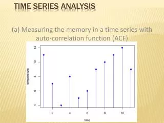
The Autocorrelation function • We identify the nature of these processes by looking at the • Autocorrelation Function (ACF), • and the Partial autocorrelation function (PACF). • These are essentially graphs of simple Pearson’s r’s calculated by correlating the variable with its lag at varying intervals. • Plots of these ACFs and PACFs reveal certain characteristic patterns for certain processes.
Identification • Visually inspect for stationarity • Difference the data if trend or drift is present. • Take logs if differenced data appears to have variance non-stationarity • Examine autocorrelations and partial autocorrelations. • Select a trial Noise model.
Estimation • Fit the trial noise model with the estimation routine. • Ensure that the parameters are significant.
Diagnosis • Ensure that the residuals are a white noise process via the 2 test. • (Note Maddalla’s objection to this test - but a significant 2 test can still be accepted as non-random residuals) • Where two models appear comparable, choose the one with the lower rmse (root mean squared error.) • If the noise model is not random, re-specify and estimate again.

