Time series modelling
Time series modelling. Marian Scott SAGES, March 2009. what is a time series?. a time series is a sequence of measurements made over time. notationally, this would commonly be written as y 1 , y 2 ,…, y i , ….y T the index i denotes the position in the sequence of observations

Time series modelling
E N D
Presentation Transcript
Time series modelling Marian Scott SAGES, March 2009
what is a time series? • a time series is a sequence of measurements made over time. • notationally, this would commonly be written as y1, y2,…, yi, ….yT • the index i denotes the position in the sequence of observations • for this early session, we will assume that the data are equally spaced-so that i is truly an index
how to plot the data a time series plot • choice of the x-axis scale • occasionally, each observation is indexed by its position in the sequence (OK if equally spaced) • alternatively, we may use the actual timescale (e.g. if an annual series, years or a daily series, then days 1-365) • or we may regard time on a continuous scale (time might be recorded in decimal form e.g. 1986.5- which would be June 1986)
How is biodiversity changing (EEA CSI 009) • Populations of common and widespread farmland bird species in 2003 are only 71% of their 1980 levels. • an annual indicator
Water quality- freshwater (CSI 020) • Concentrations of P generally decreased • Nitrate concentrations have remained constant • What are the rates of change and are they significant?
Example 2: a time series plot (daily values) the x-axis shows the actual date
Example 3- Some typical environmental series- Loch Leven (NERC-CEH)
Example 4- air quality, monitored through time (from EMEP programme) note the gaps and the rather extreme values- one strategy is to take logs
Time series data features • patterns over time (both short and long term) • often missing data- may cause problems for statistical analysis • variation, which may not be constant over time so may need to consider transformations (log)
Seasonal patterns (cycles) • in many environmental times series, we could imagine some periodicity (e.g. such as a monthly pattern in temperature) • so it is common to produce a “seasonality plot” • the index (x-axis scale) depends on the period over which the cycle repeats itself.
Example 1: daily observations, so the seasonal curve is plotted over days of the year
Example 2: Daily data- data are plotted over the days of the week
Example 3: Loch Leven, monthly data- data are plotted over the months of the year (Lowess smooth included)
what are the questions of interest? • we want to know about trends, where a trend is defined to be: • the long-term sweep of the data. • we want to know about possible seasonality (or cycles) • The seasonalcomponent of a time series describes a regular fluctuation which has a period. (The period is the time interval between consecutive peaks or troughs.)
a descriptive model • A useful descriptive model for a time series consists of 3 components: • X = Trend + Seasonal Component + Irregular Component or X = T+S+I • I is the irregular component, which is left over when the trend, and seasonal components are all accounted for. It is an irregular or random fluctuation (like residuals in regression).
smoothing a time series • In many time series, the seasonal variation can be so strong that it obscures any trend or cyclical component. However, for understanding the process being observed (and forecasting future values of the series), trends and cycles are of prime importance. Smoothing is a process designed to remove seasonality so that the long-term movements in a time series can be seen more clearly
smoothing a time series • one of the most commonly used smoothing techniques is moving average. • difficult choice: the window over which to smooth • smooth series: Yi = wkYi+k • other smoothing methods (more modern) commonly used include Lowess
smoothing a time series • LO(W)ESS, is a method that is known as locally weighted polynomial regression. At each point in the data set a low-degree polynomial is fit to a subset of the data, with explanatory variable values near the point whose response is being estimated. The polynomial is fit using weighted least squares, giving more weight to points near the point whose response is being estimated and less weight to points further away. • Many of the details of this method, such as the degree of the polynomial model and the weights, are flexible.
Example 1: water surface temperature from Jan 1981- Feb 1992 (Piegorsch)- with lowess curve
Example 1: water surface temperature- seasonal pattern by week
Example 1: water surface temperature-moving average length 52
Example 2: different smoothing technique applied to air quality data (that have been logged)
harmonic regression • another way of a) describing and b) hence being able to remove the periodic component is to use what is called harmonic regression • remember sin and cos from school?
harmonic regression • build a regression model using the sine function. sin () lies between -1 and +1, where measured in radians. • for a periodic time series Yi we can build a regression model • Yi = 0 + sin (2[ti - ]/p) + i • to make this simpler, if we assume that p is known, this can be written as a simple multiple linear regression model
harmonic regression • for a periodic time series Yi we can build a regression model • Yi = 0 + sin (2[ti - ]/p) + i • to make this simpler, • Yi = 0 + 1ci + 2si + i • where ci = cos(2ti/p) and si = sin(2ti/p)
Example 2: red curve shows the harmonic pattern (superimposed on a declining trend).
correlation through time • in many situations, we expect successive observations to show correlation at adjacent time points (most likely stronger the closer the time points are), strength of dependence usually depends on time separation or lag • for regularly spaced data, we typically make use of the autocorrelation function (ACF)
correlation through time • for regularly spaced time series, with no missing data, we define the sample mean in the usual way • then the sample autocorrelation coefficient at lag k ( 0), r(k) • correlation between original series and a version shifted back k time units • horizontal lines show approximate 95% confidence intervals for individual coefficients.
correlation through time • ACF shows a very marked cyclical pattern • interpretation of the ACF • we need to have removed both trend and seasonality • we hope that (for simplicity in subsequent modelling) that only a few correlation coefficients (at small lags) will be significant. • ACF an important diagnostic tool for time series modelling (formal models ARIMA). Formal time series models …see later session on trends • how should we remove the seasonal pattern or the trend?
differencing • a common way of removing a simple trend (eg linear) is by differencing • define a new series • Zt = Yt – Yt-1 • a common way of removing seasonality (if we know the period to be p), is to take pth differences • Zt = Yt – Yt-p
Example 1: ACF of water temperature data- difference order 12
a descriptive model • A useful descriptive model for a time series consists of 3 components: • X = Trend + Seasonal Component + Irregular Component or X = T+S+I • I is the irregular component, which is left over when the trend and seasonal components are all accounted for. It is an irregular or random fluctuation (like residuals in regression).
simple algorithm • obtain rough estimate of trend (smoothing but one not affected by seasonality): • subtract estimated trend • estimate seasonal cycle from detrended series • what is left is the irregular component, • good alternative- STL (seasonal trend lowess) decompostion (stl() command in R)
a couple of examples for you to try • for monthly temperature data • obtain the acf • use the stl() command • for dissolved oxygen in River Clyde • fit a seasonal regression model • In the final session on trend detection we will return to regression for time series.

