Time series
Time series. Characteristics. Non-independent observations (correlations structure) Systematic variation within a year (seasonal effects) Long-term increasing or decreasing level (trend) Irregular variation of small magnitude (noise). Where can time series be found?.

Time series
E N D
Presentation Transcript
Characteristics • Non-independent observations (correlations structure) • Systematic variation within a year (seasonal effects) • Long-term increasing or decreasing level (trend) • Irregular variation of small magnitude (noise)
Where can time series be found? • Economic indicators: Sales figures, employment statistics, stock market indices, … • Meteorological data: precipitation, temperature,… • Environmental monitoring: concentrations of nutrients and pollutants in air masses, rivers, marine basins,…
Time series analysis • Purpose: Estimate different parts of a time series in order to • understand the historical pattern • judge upon the current status • make forecasts of the future development
Time series regression? Let yt=(Observed) value of times series at time point t and assume a year is divided into L seasons Regession model (with linear trend): yt=0+ 1t+jsj xj,t+t where xj,t=1 if yt belongs to season j and 0 otherwise, j=1,…,L-1 and {t } are assumed to have zero mean and constant variance (2)
The parameters 0, 1, s1,…, s,L-1 are estimated by theOrdinary Least Squares method: • (b0, b1, bs1, … ,bs,L-1)=argmin {(yt – (0+ 1t+jsj xj,t)2} • Advantages: • Simple and robust method • Easily interpreted components • Normal inference (conf.intervals, hypothesis testing) directly applicable • Drawbacks: • Fixed components in model (mathematical trend function and constant seasonal components) • No consideration to correlation between observations
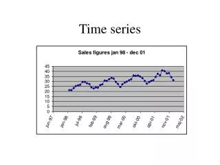
Example: Sales figures jan-98 20.33 jan-99 23.58 jan-00 26.09 jan-01 28.43 feb-98 20.96 feb-99 24.61 feb-00 26.66 feb-01 29.92 mar-98 23.06 mar-99 27.28 mar-00 29.61 mar-01 33.44 apr-98 24.48 apr-99 27.69 apr-00 32.12 apr-01 34.56 maj-98 25.47 maj-99 29.99 maj-00 34.01 maj-01 34.22 jun-98 28.81 jun-99 30.87 jun-00 32.98 jun-01 38.91 jul-98 30.32 jul-99 32.09 jul-00 36.38 jul-01 41.31 aug-98 29.56 aug-99 34.53 aug-00 35.90 aug-01 38.89 sep-98 30.01 sep-99 30.85 sep-00 36.42 sep-01 40.90 okt-98 26.78 okt-99 30.24 okt-00 34.04 okt-01 38.27 nov-98 23.75 nov-99 27.86 nov-00 31.29 nov-01 32.02 dec-98 24.06 dec-99 24.67 dec-00 28.50 dec-01 29.78
Construct seasonal indicators: x1, x2, … , x12 January (1998-2001): x1 = 1, x2 = 0, x3 = 0, …, x12 = 0 February (1998-2001): x1 = 0, x2 = 1, x3 = 0, …, x12 = 0 etc. December (1998-2001): x1 = 0, x2 = 0, x3 = 0, …, x12 = 1 Use 11 indicators, e.g. x1 - x11 in the regression model
Regression Analysis: sales versus time, x1, ... The regression equation is sales = 18.9 + 0.263 time + 0.750 x1 + 1.42 x2 + 3.96 x3 + 5.07 x4 + 6.01 x5 + 7.72 x6 + 9.59 x7 + 9.02 x8 + 8.58 x9 + 6.11 x10 + 2.24 x11 Predictor Coef SE Coef T P Constant 18.8583 0.6467 29.16 0.000 time 0.26314 0.01169 22.51 0.000 x1 0.7495 0.7791 0.96 0.343 x2 1.4164 0.7772 1.82 0.077 x3 3.9632 0.7756 5.11 0.000 x4 5.0651 0.7741 6.54 0.000 x5 6.0120 0.7728 7.78 0.000 x6 7.7188 0.7716 10.00 0.000 x7 9.5882 0.7706 12.44 0.000 x8 9.0201 0.7698 11.72 0.000 x9 8.5819 0.7692 11.16 0.000 x10 6.1063 0.7688 7.94 0.000 x11 2.2406 0.7685 2.92 0.006 S = 1.087 R-Sq = 96.6% R-Sq(adj) = 95.5%
Analysis of Variance Source DF SS MS F P Regression 12 1179.818 98.318 83.26 0.000 Residual Error 35 41.331 1.181 Total 47 1221.150 Source DF Seq SS time 1 683.542 x1 1 79.515 x2 1 72.040 x3 1 16.541 x4 1 4.873 x5 1 0.204 x6 1 10.320 x7 1 63.284 x8 1 72.664 x9 1 100.570 x10 1 66.226 x11 1 10.039
Unusual Observations Obs time sales Fit SE Fit Residual St Resid 12 12.0 24.060 22.016 0.583 2.044 2.23R 21 21.0 30.850 32.966 0.548 -2.116 -2.25R R denotes an observation with a large standardized residual Predicted Values for New Observations New Obs Fit SE Fit 95.0% CI 95.0% PI 1 32.502 0.647 ( 31.189, 33.815) ( 29.934, 35.069) Values of Predictors for New Observations New Obs time x1 x2 x3 x4 x5 x6 1 49.0 1.00 0.000000 0.000000 0.000000 0.000000 0.000000 New Obs x7 x8 x9 x10 x11 1 0.000000 0.000000 0.000000 0.000000 0.000000
Positive serial correlation: Values follow a smooth pattern Negative serial correlation: Values show a “thorny” pattern How to obtain it? Use the residuals.
Residual plot from the regression analysis: Smooth or thorny?
Durbin Watson test on residuals: Thumb rule: If d < 1 or d > 3, theconclusion is that residuals (and original data) are correlated. Use shape of figure (smooth or thorny) to decide if positive or negative) (More thorough rules for comparisons and decisions about positive or negative correlations exist.)
Durbin-Watson statistic = 2.05 (Comes in the output ) Value > 1 and < 3 No significant serial correlation in residuals!
Classical decomposition methods • Decompose – Analyse the observed time series in its different components: • Trend part (TR) • Seasonal part (SN) • Cyclical part (CL) • Irregular part (IR) Cyclical part: State-of-market in economic time series In environmental series, usually together with TR
Multiplicative model: • yt=TRt·SNt ·CLt ·IRt • Suitable for economic indicators • Level is present in TRt or in TCt=(TR∙CL)t • SNt , IRt (and CLt) works as indices Seasonal variation increases with level of yt
Additive model: • yt=TRt+SNt +CLt +IRt • More suitable for environmental data • Requires constant seasonal variation • SNt , IRt(and CLt) vary around 0
Estimation of components, working scheme • Seasonally adjustment/Deseasonalisation: • SNt usually has the largest amount of variation among the components. • The time series is deseasonalised by calculating centred and weighted Moving Averages: where L=Number of seasons within a year (L=2 for ½-year data, 4 for quaerterly data och 12 för monthly data)
Mtbecomes a rough estimate of (TR∙CL)t . • Rough seasonal components are obtained by • yt/Mt in a multiplicative model • yt – Mtin an additive model • Mean values of the rough seasonal components are calculated for eacj season separetly. L means. • The L means are adjusted to • have an exact average of 1 (i.e. their sum equals L ) in a multiplicative model. • Have an exact average of 0 (i.e. their sum equals zero) in an additive model. • Final estimates of the seasonal components are set to these adjusted means and are denoted:
The time series is now deaseasonalised by • in a multiplicative model • in an additive model where is one of depending on which of the seasons t represents.
2. Seasonally adjusted values are used to estimate the trend component and occasionally the cyclical component. If no cyclical component is present: • Apply simple linear regression on the seasonally adjusted values Estimatestrt of linear or quadratic trend component. • The residuals from the regression fit constitutes estimates, irt of the irregular component If cyclical component is present: • Estimate trend and cyclical component as a whole (do not split them) by i.e. A non-weighted centred Moving Average with length 2m+1 caclulated over the seasonally adjusted values
Common values for 2m+1: 3, 5, 7, 9, 11, 13 • Choice of m is based on properties of the final estimate of IRtwhich is calculated as • in a multiplicative model • in an additive model • m is chosen so to minimise the serial correlation and the variance of irt . • 2m+1 is called (number of) points of the Moving Average.
Example, cont: Home sales data Minitab can be used for decomposition by StatTime seriesDecomposition Val av modelltyp Option to choose between two models
Time Series Decomposition Data Sold Length 47,0000 NMissing 0 Trend Line Equation Yt = 5,77613 + 4,30E-02*t Seasonal Indices Period Index 1 -4,09028 2 -4,13194 3 0,909722 4 -1,09028 5 3,70139 6 0,618056 7 4,70139 8 4,70139 9 -1,96528 10 0,118056 11 -1,29861 12 -2,17361 Accuracy of Model MAPE: 16,4122 MAD: 0,9025 MSD: 1,6902
Deseasonalised data have been stored in a column with head DESE1. Moving Averages on these column can be calculated by StatTime seriesMoving average Choice of 2m+1
TC component with 2m +1 = 3 (blue) MSD should be kept as small as possible
By saving residuals from the moving averages we can calculate MSD and serial correlations for each choice of 2m+1. A 7-points or 9-points moving average seems most reasonable.
Serial correlations are simply calculated by StatTime seriesLag and further StatBasic statisticsCorrelation Or manually in Session window: MTB > lag ’RESI4’ c50 MTB > corr ’RESI4’ c50
Time Series Decomposition Data Sold Length 47,0000 NMissing 0 Trend Line Equation Yt = 5,77613 + 4,30E-02*t Seasonal Indices Period Index 1 0,425997 2 0,425278 3 1,14238 4 0,856404 5 1,52471 6 1,10138 7 1,65646 8 1,65053 9 0,670985 10 1,02048 11 0,825072 12 0,700325 Accuracy of Model MAPE: 16,8643 MAD: 0,9057 MSD: 1,6388
additive additive
Classical decomposition, summary Multiplicative model: Additive model:
Deseasonalisation • Estimate trend+cyclical component by a centred moving average: where L is the number of seasons (e.g. 12, 4, 2)
Filter out seasonal and error (irregular) components: • Multiplicative model: -- Additive model:
Calculate monthly averages Multiplicative model: Additive model: for seasons m=1,…,L
Normalise the monhtly means Multiplicative model: Additive model:
Deseasonalise Multiplicative model: Additive model: where snt = snm for current month m
Fit trend function, detrend (deaseasonalised) data Multiplicative model: Additive model:

