Radar Algorithms
This course by David Patrick at the Hydrometeorological and Arctic Lab in Winnipeg provides a deep dive into advanced radar algorithms essential for meteorological applications. Key topics include Doppler reflectivity, storm-relative velocity, and grid-based algorithms for severe thunderstorms. Participants will learn about cell identification, tracking, and storm assessment classification, alongside techniques for Doppler signal processing. The course highlights practical applications for operational meteorologists across Canada, emphasizing the integration of Doppler and conventional radar data for improved weather forecasting.

Radar Algorithms
E N D
Presentation Transcript
Radar Algorithms MSC Radar Course David Patrick Hydrometeorological and Arctic Lab Winnipeg, MB
Acknowledgements • Dave Ball for inspiring this course • Operational meteorologists across Canada for giving me ideas and input
Outline • Basic algorithms • PRECIP, Doppler ClogZ Reflectivity, Radial Velocity, Storm-relative Radial Velocity • Grid-based severe thunderstorm algorithms • SvrWx, CAPPI 7.0, CoTPPI, VIL, WDraft, Hail, BWER, Reflectivity Gradient, MesoCyclone, Microburst, Gust • Cell-based severe thunderstorm algorithms • Cell Identification, Cell Properties, MultiRadarMerge, Cell Tracking, Cell View, StormAssessmentClassification, SCIT
Basic Algorithms - PRECIP • PRECIP product is combo of • doppler reflectivity within 125 km • conventional reflectivity beyond 125 km doppler clutter suppression can reduce signal and create artificial boundary at 125 interface
Basic Algorithms - PRECIP 7-day Rainfall Accum • Inner doppler scan may be under-calibrated compared to outer conventional scan giving inner circle of reduced returns
Doppler & Conventional Base Reflectivity Loop • Doppler and conventional base level reflectivities are ~5 minutes apart in 10 minute scan cycle • Can create a 5-minute frequency loop by alternating between the two products (not operationally available)
Basic Algorithms Doppler vs. Conventional Reflectivity • Sometimes doppler reflectivity has holes in the data same cell with no holes in conventional data Note doppler data has 4x resolution of conventional data Doppler 0.5° “ClogZ” reflectivity Conventional 0.5° reflectivity
dBZ -VN 0 +VN Basic Algorithms – Doppler Signal Processing • At the radar site processor, a Signal Quality Index is used to determine if a radar bin’s radial velocity is good • SQI is related to • spectrum width, the degree of spread in the radial velocity elements for the radar bin; high spectrum width -> low SQI • signal to noise ratio; low signal -> low SQI • If the SQI is too low, the radial velocity is trashed, along with reflectivity! Spectrum width is measure of spread of weather ground clutter weather
Basic Algorithms – Doppler Signal Processing • Doppler data from 0.5° scan • High spectrum width causes data dropout in critical area Radial velocity Reflectivity Spectrum width signal trashed • 2010Z August 20, 2009; tornado on ground in missing data zone
Basic algorithms – Radial Velocity • Canadian radars are C-band radars (except S-band McGill) that use dual pulse repetition frequencies in doppler mode • Nyquist velocity VN is max velocity that can be unambiguously determined VN = PRF ∙ λ / 4 • All V < -VN or V > VN are “folded” into –VN to +VN range • Low PRF 892 s-1 VN = 892 ∙ 0.0534 / 4 = 11.9 m/s • High PRF 1190 s-1 VN = 1190 ∙ 0.0534 / 4 = 15.9 m/s • Low and High PRF rays are alternated around scan • Processing at radar site combines/unfolds data to give -48 m/s <= V <= +48 m/s
Basic algorithms – Radial Velocity The ‘dual-PRF’ unfolding technique • Look at relative error V1200 – V900 • Pick off actual velocity
Basic algorithms – Radial Velocity • Let’s go to SErn Newfoundland • Strong Low approaching from SW • Original folded velocities from alternating Low/High PRF rays • No V < -16 m/s or V > 16 m/s
Basic algorithms – Radial Velocity • Unfold velocities at radar site • Note bright green speckles (V= -36 m/s) embedded in yellow-pink area (V= +30 m/s) • Either bad unfolding or bad data leading to bad unfolded velocities
Basic algorithms – Radial Velocity • Corresponding analyses 1200Z Oct 17 2009 • Surface • 850 mb • 700 mb
Basic algorithms – Radial Velocity VAD winds at 0900Z Oct 17 2009 Winds are consistently from E to SE direction in lower 5,000 feet
Basic algorithms – Radial Velocity • Apply “despike” algorithm that assumes data is accurate and tries to find best unfolded velocity compared to immediate neighbours • This is what you see on the fcst desk With despike Without despike Data is smoothed but area of towards-radar velocities is increased
Basic algorithms – Radial Velocity • Try unfolding velocities at forecast office using velocity info from a wider neighbourhood (under development)
Basic Algorithms – Extra Info Long Range Radial Velocity • Note! • When looking at LongRange Velocity product, velocity folding occurs at just 16 m/s, not the usual 48 m/s • Look for light blue and orange adjacent to each other
Basic Algorithms – Storm Relative Velocity • Subtract off storm motion vector from all radial velocity bins to view motion in storm-based frame of reference Storm-based radial velocity Subtract 250/40km/h from all bins Radar-based radial velocity couplet showing away and towards motion relative to storm couplet embedded in away velocities
Grid-based Svr Wx AlgorithmsSVRWX • Based on work done by US Air Force & NSSL in 1960s and updated in Canada in 1980s • Height of 40 dBZ echo is correlated to severe weather occurrence (can be 45 dBZ in parts of Canada) • Not strongly correlated to tornadoes in high shear environments • Evidence of strong deep updraft with significant moisture/hail
Grid-based Svr Wx AlgorithmsSVRWX • SvrWx values: • 40 dBZ @ 5.5 km => level 1 blue • 40 dBZ @ 8.5 km => level 2 green • 40 dBZ @ 10.5 km => level 3 yellow • 40 dBZ @ 12.0 km => level 4 red Increasing probability of severe weather
Grid-based Svr Wx AlgorithmsSVRWX • CAPPI 1.5 km shows large swaths of strong echoes • SvrWx highlights sig convection
Grid-based Svr Wx AlgorithmsCAPPI 7.0 • CAPPI 7.0 km has traditionally been used to highlight sig cvctn • But its use depends on airmass temperature • Poor in cool airmasses
Grid-based Svr Wx AlgorithmsCoTPPI -20°C • Try using Constant Temperature PPI sfc instead of Constant Altitude PPI • -20°C sfc slides up and down with airmass • Use model data for temps not operationally available
Grid-based Svr Wx AlgorithmsVIL • Take Z for a radar bin volume, convert to liquid, and integrate thru vertical column • Shows heavy rain potential, large hail, ~ wet microburst potential • Note: VIL Density (VIL divided by depth of echoes) will partially account for a distant cell that is substantially below the lowest scan angle
Grid-based Svr Wx AlgorithmsWDRAFT • Developed by S.R. Stewart, 1991 • WDraft = 3.6 * SQRT (20.628571 x VIL - 3.125 ET**2) km/h • Algorithm looks only at instantaneous VIL and EchoTop, not rate of change of these parameters
Grid-based Svr Wx AlgorithmsWDRAFT • Big VIL packed into a relatively low echo top gives high WDraft
Grid-based Svr Wx AlgorithmsHail • Uses an algorithm developed in Southeastern Australia • Height of 50 dBZ and freezing level are empirically correlated to hail diameter • VIL and freezing level are also empirically correlated to hail diameter • Given hgt 50 dBZ, VIL and freezing level, calculate hail diameter using both methods and choose the larger of the two.
Grid-based Svr Wx AlgorithmsHail Observed Hail Size vs. Height 50 dBZ & Freezing Level
Grid-based Svr Wx AlgorithmsHail Observed Hail Size vs. VIL & Freezing Level
Grid-based Svr Wx AlgorithmsHail • Tends to over-forecast hail diameter • But in this case, 7.1 cm was good
Grid-based Svr Wx AlgorithmsHail Dauphin hailstorm Aug 9, 2007
Grid-based Svr Wx Algorithms U.S. NWS MESH & POSH Algorithms • Use a reflectivity-to-hail energy relation and integrate this energy with height above the freezing level • Using a large dataset, this integrated energy is statistically related to • MESH (Maximum Expected Size of Hail) • POSH (Probability of Severe Hail)
Grid-based Svr Wx Algorithms U.S. NWS MESH & POSH Algorithms • Hail kinetic energy E • where W(dBZ) is a weight based on reflectivity; dBZL=40, dBZU=50 0 for dBZ <= dBZL W(dBZ) = dBZ – dBZL for dBZL < dBZ < dBZU dBZU – dBZL 1 for dBZ >= dBZU
Grid-based Svr Wx Algorithms U.S. NWS MESH & POSH Algorithms • Severe Hail Index SHI • where H0 is height of fzlvl, HT is height of storm top, WT(H) is a weight based on temperature, and Hm20 (hgt -20C)All heights AboveRadarLevel 0 for H <= H0 WT(H) = H – H0 for H0 < H < Hm20 Hm20 – H0 1 for H >= Hm20
Grid-based Svr Wx Algorithms U.S. NWS MESH & POSH Algorithms • where WT is warning threshold if WT < 20, set to 20
Grid-based Svr Wx Algorithms U.S. NWS MESH & POSH Algorithms • URP Hail has +ve bias • U.S. NWS MESH no bias but underfcsts large hail; overfcsts small hail • U.S. NWS POSH if >70% svr hail likely
Grid-based Svr Wx AlgorithmsBWER (Bounded Weak Echo Region) • Find upside down cup patterns in the reflectivity volume scan, as evidence of strong updraft with rotation • Go out and up from each radar bin, looking for higher values • URP looks out in 8 directions, but up in only 5 (let’s make it 9)
Grid-based Svr Wx AlgorithmsBWER (Bounded Weak Echo Region) • Do a double pass over the data • First pass • In these 13 (try 17) directions, go out a max of 10 radar bins (try 10 km), looking for dBZ values that are at least 8 dBZ greater than the centre radar bin, and >= 40 dBZ in value (try givingpartial credit to 6+ dBZ gradients) • Count the number of “hits” • Weight all directions the same (try requiring vertical direction hit)
Grid-based Svr Wx AlgorithmsBWER (Bounded Weak Echo Region) Example: CAPPI 1.5 km XSM 0030Z July 30 2005 Rocky Mountains
Grid-based Svr Wx AlgorithmsBWER (Bounded Weak Echo Region) BWER algorithm checks out a long way in the azimuthal direction
Grid-based Svr Wx AlgorithmsBWER (Bounded Weak Echo Region) • Second pass • Go thru the first pass results, traversing the same 13 (17) directions, and subtract one “hit” every time you come across a radar bin that has a lower hit count than your centre radar bin • This gives a measure of boundedness of the centre radar bin you’re examining • Look thru the volume at all the radar bins with a non-zero hit count, and for each column of radar bins, save the height of the highest one (try saving volume as well)
Grid-based Svr Wx AlgorithmsBWER (Bounded Weak Echo Region) A final hit count of 1 or 2 is left oops
Grid-based Svr Wx AlgorithmsBWER (Bounded Weak Echo Region) Usual way to plot BWER is in white on CELL View Giant BWER
Grid-based Svr Wx AlgorithmsReflectivity Gradient • Calculates the reflectivity gradient for any specified areal product, e.g. CAPPI 1.5 km dBZ or CAPPI 3.0 km dBZ • Sharp mid-level gradients on upwind side of CB are correlated to rear-flank downdraft, mesocyclone development
Grid-based Svr Wx AlgorithmsReflectivity Gradient 3 km CAPPI dBZ 3 km dBZ Gradient Hook echo July 24 2000 2230Z Brunkild MB
Grid-based Svr Wx AlgorithmsMesocyclone • Doppler data is available for the 0.5, 1.5 and 3.5 degree elevation angles at every 0.5 km in range out to 112.5 km, and every 0.5 degrees azimuth around the radar; 225 x 720 bins • Rays alternate between low PRF and high PRF • Choose only high PRF (VN=16 m/s) rays • For every range bin away from the radar out to 225 bins, go around 360 degrees, looking for aziumthal shear across every 2nd bin, i.e. every high PRF ray • Note zones of strong connected bin-to-bin (gate-to-gate) azimuthal shear over the 3 scan angles and group them into “features”.
Grid-based Svr Wx AlgorithmsMesocyclone • If feature has too little • area, • shear less than min shear threshold, • higher shear but weak momentum, or • dBZ • then trash. • These thresholds are configurable.
Grid-based Svr Wx AlgorithmsMesocyclone • Assigning levels • Level 1 => 1 meso detected at 1.5 or 3.5 degrees • Level 2 => 2 mesos detected at 1.5 & 3.5 degrees • Level 3 => mesos detected at all 3 levels OR meso detected at lowest 0.5 degree level • Level 4 => a level 3 that has sufficient momentum and max gate-to-gate shear • Level 5 => a level 4 that is at least 5 km across in the radial direction? • Assigning circle diameter • Seems that the circle diameter is related to the diameter of the circulation in the azimuthal direction … 10 times? diameter
Grid-based Svr Wx AlgorithmsMesocyclone • Strong mesocyclone NW of Kitchener/ Waterloo • Tornado on ground at time WSO Kitchener Hwy 401