Understanding Spectroscopy: Quantum Numbers, Spectral Lines, and Atomic Transitions
This comprehensive overview of spectroscopy delves into the principles of spectral lines and the Fraunhofer spectrum, discussing key concepts such as quantum numbers, electron transitions, and the notation used in spectroscopy. It highlights the different types of quantum states (s, p, d, f) and explores how electron transitions occur via allowed and forbidden methods. Important phenomena such as the Pauli exclusion principle, metastable states, doppler and collisional broadening, and classical radiation models are also elaborated upon, providing a well-rounded understanding of atomic structure and light interaction.

Understanding Spectroscopy: Quantum Numbers, Spectral Lines, and Atomic Transitions
E N D
Presentation Transcript
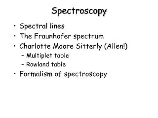
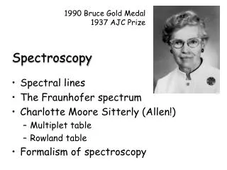
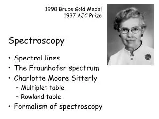
Spectroscopy 1990 Bruce Gold Medal 1937 AJC Prize • Spectral lines • The Fraunhofer spectrum • Charlotte Moore Sitterly • Multiplet table • Rowland table • Formalism of spectroscopy
Quantum Numbers of Atomic States • Principal quantum number n defines the energy level • Azimuthal quantum number l • states with l=0 called s states • states with l=1 called p states • states with l=2 called d states • states with l=3 called f states • “orbits” of s states become more eccentric as n increases • Electron transitions take place between adjacent angular momentum states (i.e. Dl=1) • “sharp series” lines from p to higher s states • “principal series” lines from s to higher p states • “diffuse series” lines from p to higher d states • “fundamental series” lines from d to higher f states • The first line(s) of the principal series (s to p) are called resonance lines since it involves the ground level • In alkali metals, the p, d, and f energy levels are doubled (e.g. the Na D lines) due to the coupling between the magnetic moment of the orbital motion and the spin of the electron (the quantum number s, which can be +1/2 or –1/2
Spectroscopic Notation • The total angular momentum quantum number is j • For s states, j=1/2 • For p states, j=1/2 or j=3/2 • Electron levels are designated by the notation “n2(L)J” • n is the total quantum number • The superscript 2 indicates the levels are doubled • L is the azimuthal quantum number (S,P,D,F) • J denotes the angular momentum quantum number • For the sodium ground level is 3s2S1/2 • The two lowest p levels are 3p2P1/2 and 3p2P 3/2 • The Na D lines are described • 3s2S½ - 3p2P3/2 l5889.953 and 3s2S½ - 3p2P1/2l5895.923 * This is a different S than the s state!
More Spectroscopic Vocabulary • The Pauli exclusion principle requires that two s-electrons in the same state must have opposite spin • Therefore S=0 and these are called “singlet” states • The ground state of He is a singlet state – 1S0 • The superscript 1 means singlet • The subscript 0 means J=0 • In the first excited state of He, one electron is in the 1s state, and the second can be in either the 2s or the 2p state. • Depending on how the electrons’ spins are aligned, these states can either be singlets or triplets • Electrons can only jump between singlet states or between triplet states
It goes on and on and on… • The state of the electrons is described with a term for each electron above the closed shell. • For carbon atoms, “1s22s22p2”says there are • 2 electrons in the 1s state • 2 electrons in the 2s state • 2 electrons in the 2p state • Allowed and forbidden transitions • Transitions with Dl=1 and DJ=1 and 0 are allowed (except between J=0 and J=0) • Other transitions are forbidden • For some electron states there are no allowed transitions to lower energy states. Such levels are called metastable • The situation is more complex in atoms with more electrons • A multiplet is the whole group of transitions between two states, say 3P-3D
Grotrian Diagram for He • Struve and Wurm 1938, ApJ
Spectral Line Formation • Classical picture of radiation • Intrinsic vs. extrinsic broadening mechanisms • Line absorption coefficient • Radiative transfer in spectral lines
Spectral Line Formation-Line Absorption Coefficient • Radiation damping (atomic absorptions and emissions aren’t perfectly monochromatic – uncertainty principle) • Thermal broadening from random kinetic motion • Collisional broadening – perturbations from neighboring atoms/ions/electrons) • Hyperfine structure • Zeeman effect
Classical Picture of Radiation • Photons are sinusoidal variations of electro-magnetic fields • When a photon passes by an electron in an atom, the changing fields cause the electron to oscillate • Treat the electron as a classical harmonic oscillator: mass x acceleration = external force – restoring force – dissipative • E&M is useful! (well…)
Atomic Absorption Coefficient • N0 is the number of bound electrons per unit volume • the quantity n-n0 is the frequency separation from the nominal line center • the quantity e is the dielectric constant (e=1 in free space) • and g=g/m is the classical damping constant The atomic absorption coefficient includes atomic data (f, e, g) and the state of the gas (N0), and is a function of frequency. The equation expresses the natural broadening of a spectral line.
The Classical Damping Constant • For a classical harmonic oscillator, • The shape of the spectral line depends on the size of the classical damping constant • For n-n0 >> g/4p, the line falls off as (n-n0)-2 • Accelerating electric charges radiate. • and • is the classical damping constant (l is in cm) The mean lifetime is also defined as T=1/g, where T=4.5l2
The Classical Line Profile • Look at a thin atmospheric layer between t2 (the deeper layer) and t1 • The line profile is proportional to kn • At line center n=n0, and • Half the maximum depth occurs at (n-n0)=g/4p • In terms of wavelength • Very small – and the same for ALL lines!
An example… • The Na D lines have a wavelength of 5.9x10⁻⁵ cm. g = 6.4 x 10⁷ sec-1 • The absorption coefficient per gram of Na atoms at a distance of 2A from line center can be calculated: Dn0-n = 1.7 x 10¹¹ sec-1 and N = 1/m = 2.6 x 10²² atoms gm-1 • Then k = 3.7 x 10⁴f • and f=2/3, so k = 2.5 x 10⁴ per gram of neutral sodium
The Abundance of Sodium • In the Sun, the Na D lines are about 1% deep at a distance of 2A from line center • Use a simple one-layer model of depth x (the Schuster-Schwarzschild model) • Or krx=0.01, and rx=4x10⁻⁷ gm cm-2 (recall thatkNa=2.5 x 10⁴ per gram of neutral sodium at a distance of 2A from line center) • the quantity rx is a column density
Natural Broadening • From Heisenberg's uncertainty principle: The electron in an excited state is only there for a short time, so its energy cannot have a precise value. • Since energy levels are "fuzzy," atoms can absorb photons with slightly different energy, with the probability of absorption declining as the difference in the photon's energy from the "true" energy of the transition increases. • The FWHM of natural broadening for a transition with an average waiting time of Dto is given by • A typical value of (Dl)1/2 = 2 x 10⁻⁴ A. Natural broadening is usually very small. • The profile of a naturally broadened linen is given by a dispersion profile (also called a damping profile, a Lorentzian profile, a Cauchy curve, and the Witch of Agnesi!) of the form (in terms of frequency) • where g is the "damping constant."
The Classical Damping Constant • For a classical harmonic oscillator, • The shape of the spectral line depends on the size of the classical damping constant • For n-n0 >> g/4p, the line falls off as (n-n0)-2 • Accelerating electric charges radiate. • and • is the classical damping constant (l is in cm) The mean lifetime is also defined as T=1/g, where T=4.5l2
Line Absorption with QM • Replace g with G! • Broadening depends on lifetime of level • Levels with long lifetimes are sharp • Levels with short lifetimes are fuzzy • QM damping constants for resonance lines may be close to the classical damping constant • QM damping constants for other Fraunhofer lines may be 5,10, or even 50 times bigger than the classical damping constant
Add Quantum Mechanics • Define the oscillator strength, f: • related to the atomic transition probability Bul: • f-values usually tabulated as gf-values. • theoretically calculated • laboratory measurements • solar
Collisional Broadening • Perturbations by discrete encounters • Change in energy approximated by a power law of the form DE = constant x r-n (r is the separation between the atom and the perturber) • Perturbations by static ion fields (linear Stark effect broadening) (n=2) • Self-broadening - collisions with neutral atoms of the same kind (resonance broadening, n=3) • if perturbed atom or ion has an inner core of electrons (i.e. with a dipole moment) (quadratic Stark effect, n=4) • Collisions with atoms of another kind (neutral hydrogen atoms) (van der Waals, n=6) • Assume adiabatic encounters (electron doesn’t change level) • Non-adiabatic (electron changes level) collisions also possible
Approaches to Collisional Broadening • Statistical effects of many particles (pressure broadening) • Usually applies to the wings, less important in the core • Some lines can be described fully by one or the other • Know your lines! • The functional form for collisional damping is the same as for radiation damping, but Grad is replaced with Gcoll • Collisional broadening is also described with a dispersion function • Collisional damping is sometimes 10’s of times larger than radiation damping
Doppler Broadening • Two components contribute to the intrinsic Doppler broadening of spectral lines: • Thermal broadening • Turbulence – the dreaded microturbulence! • Thermal broadening is controlled by the thermal velocity distribution (and the shape of the line profile) where vr is the line of sight velocity component • The Doppler width associated with the velocity v0 (where the variance v02=2kT/m) is and l is the wavelength of line center
More Doppler Broadening • Combining these we get the thermal broadening line profile: • At line center, n=n0, and this reduces to • Where the line reaches half its maximum depth, the total width is
Thermal + Turbulence • The average speed of an atom in a gas due to thermal motion - Maxwell Boltzmann distribution. The most probably speed is given by • Moving atoms are Doppler shifted, and individual atoms will absorb light at slightly different wavelengths because of the Doppler shift. • Spectral lines are also Doppler broadened by turbulent motions in the gas. The combination of these two effects produces a Doppler-broadened profile: • Typical values for Dl1/2 are a few tenths of an Angstrom. The line depth for Doppler broadening decreases exponentially from the line center.
Combining the Natural, Collisional and Thermal Broadening Coefficients • The combined broadening coefficient is just the convolution of all of the individual broadening coefficients • The natural, Stark, and van der Waals broadening coefficients all have the form of a dispersion profile: • With damping constants (grad, g2, g4, g6) one simply adds them up to get the total damping constant: • The thermal profile is a Gaussian profile:
The Voigt Profile • The convolution of a dispersion profile and a Gaussian profile is known as a Voigt profile. • Voigt functions are tabulated for use in computation • In general, the shapes of spectra lines are defined in terms of Voigt profiles • Voigt functions are dominated by Doppler broadening at small Dl, and by radiation or collisional broadening at large Dl • For weak lines, it’s the Doppler core that dominates. • In solar-type stars, collisions dominate g, so one needs to know the damping constant and the pressure to compute the line absorption coefficient • For strong lines, we need to know the damping parameters to interpret the line.
Calculating Voigt Profiles • Tabulated as the Hjerting function H(u,a) • u=Dl/DlD • a=(l2/4pc)/DlD =(g/4p)DnD • Hjertung functions are expanded as: H(u,a)=H0(u) + aH1(u) + a2H2(u) + a3H3(u) +… • or, the absorption coefficient is