Download
1 / 49
490 likes | 776 Vues
STAT131 W 11 L 1a: Comparing t w o populations. by Anne Porter alp@uow.edu.au. Comparing populations. Comparing two proportions n large Z Comparing two means n large s known Z s unknown estimated by s t n small but normally distributed data s known Z

E N D
STAT131W11L1a: Comparing two populations by Anne Porter alp@uow.edu.au
Comparing populations • Comparing two proportions • n large Z • Comparing two means • n large • s known Z • s unknown estimated by s t • n small but normally distributed data • s known Z • s unknown estimated by s t
Comparing two means Measurements are from two independent random samples Use of the Normal (Z) or t distribution Choice pertains to assumptions • s1 and s2 known or unknown AND • Small n AND both populations normally distributed OR • Large n
s1 and s2 known Confidence intervals for the difference in means Calculating Z for the hypothesis test
t-test s1 and s2 unknown(the more general case) • (s1 and s2 estimated by S1 and S2) • AND • Small n AND both populations normally distributed • OR • Large n Confidence Interval
Estimates of standard deviation for the difference between two sample means Two sample variances considered to be equal (pooled) Two sample variances considered unequal (unpooled)
Degrees of freedom df= v are given by • Two sample variances considered to be equal df= v=n1+ n2-2 • Two sample variances considered unequal dfcan be approximated by v= minimum (n1-1, n2-1) Rather than
Comparing two population means • Test at the 5% level of significance to see if there is a difference in the mean level of blood pressure for men and women • Find the 95% CI for the difference in two means
SPSS Output –making sense of data Females have a higher mean blood pressure reading than males and possibly a Lower spread. Are these differences sufficiently small to be considered to have occurred by chance if there is no real difference?
Checking assumptions for t-test • Independence - usually by design • Eg males versus females • Not independent • students with a time 1 and time 2 test scores • twins with randomly assigned one to each group
Normality BP Stem-and-Leaf Plot for SEX= m Frequency Stem & Leaf 3.00 10 . 899 1.00 11 . 4 3.00 12 . 045 8.00 13 . 23444569 2.00 14 . 09 2.00 15 . 27 2.00 Extremes (>=164) Stem width: 10.00 Each leaf: 1 case(s)Extreme It is difficult to see with small data sets but these could be interpreted as reasonably normally distributed
Normality BP Stem-and-Leaf Plot forSEX= f Frequency Stem & Leaf 2.00 11 . 69 4.00 12 . 0356 9.00 13 . 444556999 4.00 14 . 0266 3.00 15 . 179 2.00 16 . 33 1.00 Extremes (>=166) Stem width: 10.00 Each leaf: 1 case(s) It is difficult to see with small data sets but these could be interpreted as reasonably normally distributed
Normal Q-Q Plot Process • Determine the normal scores of the sample • (Z scores expected from smallest to largest in a sample this size) • Sample value plotted against its normal score Points are meant to fall on a straight line if normally distributed
Normal Q-Q Plot • How straight does the line need to be? Examine this by simulating samples with the same size and same population parameters
Equal variances – This shows Range and IQR Spread looks similar Why? Ranges approximately equal IQR close (not one twice the other
P-value>.05 therefore No evidence to suggest Unequal variances SPSS Output V11
Formally Step 1: Specify hypotheses Step 2: Specify a Step 3: Decide on the statistic and region of rejection Check normality of both samples --OK Check variances equal or unequal -- Levene’s (can look at boxplot). The test for equality of variances is not significant as p-value= 0.586 Hence t with equal variances and df=n1+n2-2If |t| >see t tables Step 4: Calculate t Step 5 Conclude
Variances assumed equal t=1.176 >tdf,a/2 as probability of getting a t as extreme as this is 0.246 ie >.025 Hence no reason to reject Ho SPSS Output V11
Verify the value of t SPSS Output V11
Conclude • As p-value =.246 ie p is higher than .05 we have no reason to reject H0 • OR • As |-1.176| < See t tables We have no evidence to suggest that there is any difference in blood pressure for males and females
Testing using 95% confidence interval As the difference in means is hypothesised to be 0 and this lies within The confidence interval there is no reason to reject Ho.
Comparing two population means • Test at the 5% level of significance to see if there is a difference in the mean weight loss for two samples. Subjects were randomly assigned to one of two different diets. • Find the 95% CI for the difference in two means
Look at the data: what does it suggest? • The variable is normal if the points fall on a straight line - it is difficult to assess so why not look at some simulated samples
Look at the data: what does it suggest? WEIGHT Stem-and-Leaf Plot forGROUP= 2.00 Frequency Stem & Leaf 2.00 2 . 79 3.00 3 . 005 1.00 4 . 1 4.00 5 . 1238 6.00 6 . 001178 3.00 7 . 779 3.00 8 . 457 2.00 9 . 02 1.00 10 . 4 Stem width: 1.00 Each leaf: 1 case(s) Looks reasonably Normal - it is hard To tell with small samples
Look at the data: what does it suggest? WEIGHT Stem-and-Leaf Plot for GROUP= 1.00 Frequency Stem & Leaf 1.00 -0 . 2 6.00 0 . 011223 12.00 0 . 566778888899 2.00 1 . 23 Stem width: 10.00 Each leaf: 1 case(s) Looks reasonably Normal - it is hard To tell with small samples
The probability of getting an F statistic as large as this if there is no differences in variances is 0.006 ie variances are different so use SPSS V10 output • As the probability of getting this t of -.11 is high (p-value =.910) ie greater than 0.05 then we retain H0 there appears to be no difference in mean weight loss
SPSS V11output – different layoutAnalyse, Compare means, independent samples, etc
Checking assumptions for t-test • What if we do not have independent groups • That is a two-sample t-test • Examples • students with a time 1 and time 2 test scores • twins with randomly assigned one to each group • Data are paired or matched • Analysis takes into account correlation between the two measures
Paired t-test Using d to represent the difference between x1- x2 • Ho: md = 0 • Ha: md ≠ 0 • Select a • Select test and state decision rule for rejection • Calculate test statistic as for one sample t on diff • Draw conclusions
Data Utts, p446. Time for task performance By 10 pilots under Alcohol and no alcohol Conditions. Diff is the time difference No alcohol - alcohol
Examine plots of both variables One outlier in the alcohol condition. The median time is lower for the alcohol condition (300) than no alcohol. The spread (IQR)is greater for the noalcohol condition. Some asymmetry in both conditions. N is small.
Menu options • Analyse, Compare Means, Paired Samples T-test • Must select two variables to move to paired analysis OR • Analyse, Compare Means, One sample t, analysing the variable diff
Check Assumptions – Normality for n is small DIFF Stem-and-Leaf Plot Frequency Stem & Leaf 2.00 -0 . 00 6.00 0 . 000113 2.00 0 . 55 Stem width: 1000 Each leaf: 1 case(s)
Output – two tailed Ha: m≠0 t =2.286 >t9,0.025 The probability of getting a t this extreme is 0.025 As this is low, <.05, there is evidence that the means times are not the same for the alcohol and no alcohol groups.
Output – one tailed Ha: m>0 As the probability of a t this large is 0.025/2 (one tailed)=0.0125, that is smaller than .05 we reject Ho there is evidence that the mean times are not the same. (Note in Utts the Minitab p is the one tail value and doubled if two tailed)
Comparing two proportions From central limit theorem, n large >30 can use Normal(Z) distribution. Samples must be independent, and for both samples at least 5, preferably 10. Confidence Interval for difference in proportions Test Statistic
Example • A survey of people in NSW revealed the following voting intentions.
Example • (1) Find the 95% confidence interval for the difference in proportions of males and females voting alp
CI for difference -assumptions should be more than 10
CI for difference in two proportions As 0 lies between the upper and lower limits of the CI we can conclude that there is no real difference between the Males and female proportion of alp voters.
Example – Hypothesis Test Ho: Ha: a= Decision Calculate From before
Example – Hypothesis Test Ho: pm= pf Ha: pm≠ pf a=.05 Decision if |Z|>1.96 reject H0 Calculate From before
Example – Hypothesis Test Conclusion As 1.45 < 1.96 there is no reason to reject Ho that the proportions of male alp voters is different to the proportion of female alp voters
Formal Steps • Specify hypotheses • Specify Alpha • Select test and rejection region • Compute statistic from data • Draw conclusions
Comparing three means • Not by multiple t-tests • Analysis of Variance techniques see Chapter 16, p561-576
Comparing three medians • Not by multiple t-tests • Non-parametric procedures See Utts Section 16.3