Bayesian models as a tool for revealing inductive biases
440 likes | 622 Vues
Bayesian models as a tool for revealing inductive biases. Tom Griffiths University of California, Berkeley. Learning languages from utterances. blicket toma dax wug blicket wug. S X Y X {blicket,dax} Y {toma, wug}. Learning functions from ( x , y ) pairs.

Bayesian models as a tool for revealing inductive biases
E N D
Presentation Transcript
Bayesian models as a tool for revealing inductive biases Tom Griffiths University of California, Berkeley
Learning languages from utterances blicket toma dax wug blicket wug S X Y X {blicket,dax} Y {toma, wug} Learning functions from (x,y) pairs Learning categories from instances of their members Inductive problems
Revealing inductive biases • Many problems in cognitive science can be formulated as problems of induction • learning languages, concepts, and causal relations • Such problems are not solvable without bias (e.g., Goodman, 1955; Kearns & Vazirani, 1994; Vapnik, 1995) • What biases guide human inductive inferences? How can computational models be used to investigate human inductive biases?
Models and inductive biases • Transparent
Bayesian models Reverend Thomas Bayes
Likelihood Prior probability Posterior probability Sum over space of hypotheses Bayes’ theorem h: hypothesis d: data
Three advantages of Bayesian models • Transparent identification of inductive biases through hypothesis space, prior, and likelihood • Opportunity to explore a range of biases expressed in terms that are natural to the problem at hand • Rational statistical inference provides an upper bound on human inferences from data
Two examples Causal induction from small samples (Josh Tenenbaum, David Sobel, Alison Gopnik) Statistical learning and word segmentation (Sharon Goldwater, Mark Johnson)
Two examples Causal induction from small samples (Josh Tenenbaum, David Sobel, Alison Gopnik) Statistical learning and word segmentation (Sharon Goldwater, Mark Johnson)
See this? It’s a blicket machine. Blickets make it go. Let’s put this one on the machine. Oooh, it’s a blicket! Blicket detector (Dave Sobel, Alison Gopnik, and colleagues)
“One cause” (Gopnik, Sobel, Schulz, & Glymour, 2001) • Two objects: A and B • Trial 1: A B on detector – detector active • Trial 2: B on detector – detector inactive • 4-year-olds judge whether each object is a blicket • A: a blicket (100% say yes) • B: almost certainly not a blicket (16% say yes) A Trial B Trial AB Trial A B
Hypotheses: causal models A B A B A B A B E E E E Defines probability distribution over variables (for both observation, and intervention) (Pearl, 2000; Spirtes, Glymour, & Scheines, 1993)
Prior and likelihood: causal theory • Prior probability an object is a blicket is q • defines a distribution over causal models • Detectors have a deterministic “activation law” • always activate if a blicket is on the detector • never activate otherwise (Tenenbaum & Griffiths, 2003; Griffiths, 2005)
Prior and likelihood: causal theory P(h00) = (1 – q)2 P(h01) = (1 – q) q P(h10) = q(1 – q) P(h11) = q2 A B A B A B A B E E E E P(E=1 | A=0, B=0): 0 0 0 0 P(E=0 | A=0, B=0): 1 1 1 1 P(E=1 | A=1, B=0): 0 0 1 1 P(E=0 | A=1, B=0): 1 1 0 0 P(E=1 | A=0, B=1): 0 1 0 1 P(E=0 | A=0, B=1): 1 0 1 0 P(E=1 | A=1, B=1): 0 1 1 1 P(E=0 | A=1, B=1): 1 0 0 0
Modeling “one cause” P(h00) = (1 – q)2 P(h01) = (1 – q) q P(h10) = q(1 – q) P(h11) = q2 A B A B A B A B E E E E P(E=1 | A=0, B=0): 0 0 0 0 P(E=0 | A=0, B=0): 1 1 1 1 P(E=1 | A=1, B=0): 0 0 1 1 P(E=0 | A=1, B=0): 1 1 0 0 P(E=1 | A=0, B=1): 0 1 0 1 P(E=0 | A=0, B=1): 1 0 1 0 P(E=1 | A=1, B=1): 0 1 1 1 P(E=0 | A=1, B=1): 1 0 0 0
Modeling “one cause” P(h01) = (1 – q) q P(h10) = q(1 – q) P(h11) = q2 A B A B A B E E E P(E=1 | A=0, B=0): 0 0 0 0 P(E=0 | A=0, B=0): 1 1 1 1 P(E=1 | A=1, B=0): 0 0 1 1 P(E=0 | A=1, B=0): 1 1 0 0 P(E=1 | A=0, B=1): 0 1 0 1 P(E=0 | A=0, B=1): 1 0 1 0 P(E=1 | A=1, B=1): 0 1 1 1 P(E=0 | A=1, B=1): 1 0 0 0
Modeling “one cause” P(h10) = q(1 – q) A B A is definitely a blicket B is definitely not a blicket E P(E=1 | A=0, B=0): 0 0 0 0 P(E=0 | A=0, B=0): 1 1 1 1 P(E=1 | A=1, B=0): 0 0 1 1 P(E=0 | A=1, B=0): 1 1 0 0 P(E=1 | A=0, B=1): 0 1 0 1 P(E=0 | A=0, B=1): 1 0 1 0 P(E=1 | A=1, B=1): 0 1 1 1 P(E=0 | A=1, B=1): 1 0 0 0
“One cause” (Gopnik, Sobel, Schulz, & Glymour, 2001) • Two objects: A and B • Trial 1: A B on detector – detector active • Trial 2: B on detector – detector inactive • 4-year-olds judge whether each object is a blicket • A: a blicket (100% say yes) • B: almost certainly not a blicket (16% say yes) A Trial B Trial AB Trial A B
Building on this analysis • Transparent
Other physical systems From stick-ball machines… …to lemur colonies (Kushnir, Schulz, Gopnik, & Danks, 2003) (Griffiths, Baraff, & Tenenbaum, 2004) (Griffiths & Tenenbaum, 2007)
Two examples Causal induction from small samples (Josh Tenenbaum, David Sobel, Alison Gopnik) Statistical learning and word segmentation (Sharon Goldwater, Mark Johnson)
Bayesian segmentation • In the domain of segmentation, we have: • Data: unsegmented corpus (transcriptions). • Hypotheses: sequences of word tokens. • Optimal solution is the segmentation with highest prior probability = 1 if concatenating words forms corpus, = 0 otherwise. Encodes assumptions about the structure of language
Brent (1999) • Describes a Bayesian unigram model for segmentation. • Prior favors solutions with fewer words, shorter words. • Problems with Brent’s system: • Learning algorithm is approximate (non-optimal). • Difficult to extend to incorporate bigram info.
A new unigram model (Dirichlet process) Assume word wi is generated as follows: 1. Is wi a novel lexical item? Fewer word types = Higher probability
A new unigram model (Dirichlet process) Assume word wi is generated as follows: 2.If novel, generate phonemic form x1…xm : If not, choose lexical identity of wi from previously occurring words: Shorter words = Higher probability Power law = Higher probability
Unigram model: simulations • Same corpus as Brent (Bernstein-Ratner, 1987): • 9790 utterances of phonemically transcribed child-directed speech (19-23 months). • Average utterance length: 3.4 words. • Average word length: 2.9 phonemes. • Example input: yuwanttusiD6bUk lUkD*z6b7wIThIzh&t &nd6dOgi yuwanttulUk&tDIs ...
What happened? • Model assumes (falsely) that words have the same probability regardless of context. • Positing amalgams allows the model to capture word-to-word dependencies. P(D&t) = .024 P(D&t|WAts) = .46 P(D&t|tu) = .0019
What about other unigram models? • Brent’s learning algorithm is insufficient to identify the optimal segmentation. • Our solution has higher probability under his model than his own solution does. • On randomly permuted corpus, our system achieves 96% accuracy; Brent gets 81%. • Formal analysis shows undersegmentation is the optimal solution for any (reasonable) unigram model.
Bigram model (hierachical Dirichlet process) Assume word wi is generated as follows: • Is (wi-1,wi) a novel bigram? • If novel, generate wi using unigram model (almost). If not, choose lexical identity of wi from words previously occurring after wi-1.
Conclusions • Both adults and children are sensitive to the nature of mechanisms in using covariation • Both adults and children can use covariation to make inferences about the nature of mechanisms • Bayesian inference provides a formal framework for understanding how statistics and knowledge interact in making these inferences • how theories constrain hypotheses, and are learned
A probabilistic mechanism? • Children in Gopnik et al. (2001) who said that B was a blicket had seen evidence that the detector was probabilistic • one block activated detector 5/6 times • Replace the deterministic “activation law”… • activate with p = 1- if a blicket is on the detector • never activate otherwise
Deterministic vs. probabilistic Deterministic mechanism knowledge affects intepretation of contingency data Probability of being a blicket Probabilistic One cause
A B Manipulating mechanisms I. Familiarization phase: Establish nature of mechanism same block At end of the test phase, adults judge the probability that each object is a blicket II. Test phase: one cause B Trial AB Trial
Bayes People Manipulating mechanisms(n = 12 undergraduates per condition) Deterministic Probability of being a blicket Probabilistic One cause
Bayes People Manipulating mechanisms (n = 12 undergraduates per condition) Deterministic Probability of being a blicket Probabilistic One control One cause Three control
A B Acquiring mechanism knowledge I. Familiarization phase: Establish nature of mechanism same block At end of the test phase, adults judge the probability that each object is a blicket II. Test phase: one cause B Trial AB Trial
Results with children • Tested 24 four-year-olds (mean age 54 months) • Instead of rating, yes or no response • Significant difference in one cause B responses • deterministic: 8% say yes • probabilistic: 79% say yes • No significant difference in one control trials • deterministic: 4% say yes • probabilistic: 21% say yes (Griffiths & Sobel, submitted)
Comparison to previous results • Proposed boundaries are more accurate than Brent’s, but fewer proposals are made. • Result: word tokens are less accurate. Precision: #correct / #found= [= hits / (hits + false alarms)] Recall: #found / #true = [= hits / (hits + misses)] F-score: an average of precision and recall.
Quantitative evaluation • Compared to unigram model, more boundaries are proposed, with no loss in accuracy: • Accuracy is higher than previous models:
Two examples Causal induction from small samples (Josh Tenenbaum, David Sobel, Alison Gopnik) Statistical learning and word segmentation (Sharon Goldwater, Mark Johnson)