Bayesian models of human inductive learning
740 likes | 768 Vues
Bayesian models of human inductive learning. Josh Tenenbaum MIT. Everyday inductive leaps. How can people learn so much about the world from such limited evidence? Kinds of objects and their properties The meanings of words, phrases, and sentences Cause-effect relations

Bayesian models of human inductive learning
E N D
Presentation Transcript
Bayesian models of human inductive learning Josh Tenenbaum MIT
Everyday inductive leaps How can people learn so much about the world from such limited evidence? • Kinds of objects and their properties • The meanings of words, phrases, and sentences • Cause-effect relations • The beliefs, goals and plans of other people • Social structures, conventions, and rules “tufa”
Modeling Goals • Explain how and why human learning and reasoning works, in terms of (approximations to) optimal statistical inference in natural environments. • Computational-level theories that provide insights into algorithmic- or processing-level questions. • Principled quantitative models of human behavior, with broad coverage and a minimum of free parameters and ad hoc assumptions. • A framework for studying people’s implicit knowledge about the world: how it is structured, used, and acquired. • A two-way bridge to state-of-the-art AI, machine learning.
Explaining inductive learning 1. How does background knowledge guide learning from sparsely observed data? Bayesian inference, with priors based on background knowledge. 2. What form does background knowledge take, across different domains and tasks? Probabilities defined over structured representations: graphs, grammars, rules, logic, relational schemas, theories. 3. How is background knowledge itself learned? Hierarchical Bayesian models, with inference at multiple levels of abstraction. 4. How can background knowledge constrain learning yet maintain flexibility, balancing assimilation and accommodation?Nonparametric models, growing in complexity as the data require.
Two case studies • The number game • Property induction
The number game • Program input: number between 1 and 100 • Program output: “yes” or “no”
The number game • Learning task: • Observe one or more positive (“yes”) examples. • Judge whether other numbers are “yes” or “no”.
The number game Examples of “yes” numbers Generalization judgments (N = 20) 60 Diffuse similarity
The number game Examples of “yes” numbers Generalization judgments (N = 20) 60 Diffuse similarity 60 80 10 30 Rule: “multiples of 10”
The number game Examples of “yes” numbers Generalization judgments (N = 20) 60 Diffuse similarity 60 80 10 30 Rule: “multiples of 10” Focused similarity: numbers near 50-60 60 52 57 55
The number game Examples of “yes” numbers Generalization judgments (N = 20) 16 Diffuse similarity 16 8 2 64 Rule: “powers of 2” Focused similarity: numbers near 20 16 23 19 20
60 Diffuse similarity 60 80 10 30 Rule: “multiples of 10” Focused similarity: numbers near 50-60 60 52 57 55 The number game Main phenomena to explain: • Generalization can appear either similarity-based (graded) or rule-based (all-or-none). • Learning from just a few positive examples.
Divisions into “rule” and “similarity” subsystems? • Category learning • Nosofsky, Palmeri et al.: RULEX • Erickson & Kruschke: ATRIUM • Language processing • Pinker, Marcus et al.: Past tense morphology • Reasoning • Sloman • Rips • Nisbett, Smith et al.
Bayesian model • H: Hypothesis space of possible concepts: • h1 = {2, 4, 6, 8, 10, 12, …, 96, 98, 100} (“even numbers”) • h2 = {10, 20, 30, 40, …, 90, 100} (“multiples of 10”) • h3 = {2, 4, 8, 16, 32, 64} (“powers of 2”) • h4 = {50, 51, 52, …, 59, 60} (“numbers between 50 and 60”) • . . . Representational interpretations for H: • Candidate rules • Features for similarity • “Consequential subsets” (Shepard, 1987)
Three hypothesis subspaces for number concepts • Mathematical properties (24 hypotheses): • Odd, even, square, cube, prime numbers • Multiples of small integers • Powers of small integers • Raw magnitude (5050 hypotheses): • All intervals of integers with endpoints between 1 and 100. • Approximate magnitude (10 hypotheses): • Decades (1-10, 10-20, 20-30, …)
Bayesian model • H: Hypothesis space of possible concepts: • Mathematical properties: even, odd, square, prime, . . . . • Approximate magnitude: {1-10}, {10-20}, {20-30}, . . . . • Raw magnitude: all intervals between 1 and 100. • X = {x1, . . . , xn}: n examples of a concept C. • Evaluate hypotheses given data: • p(h) [prior]: domain knowledge, pre-existing biases • p(X|h) [likelihood]: statistical information in examples. • p(h|X) [posterior]: degree of belief that h is the true extension of C.
Generalizing to new objects Given p(h|X), how do we compute , the probability that C applies to some new stimulus y? Background knowledge h X = x1x2 x3 x4
Generalizing to new objects Hypothesis averaging: Compute the probability that C applies to some new object y by averaging the predictions of all hypotheses h, weighted by p(h|X):
Likelihood: p(X|h) • Size principle: Smaller hypotheses receive greater likelihood, and exponentially more so as n increases. • Follows from assumption of randomly sampled examples + law of “conservation of belief”: • Captures the intuition of a “representative” sample.
Illustrating the size principle h1 2 4 6 8 10 12 14 16 18 20 22 24 26 28 30 32 34 36 38 40 42 44 46 48 50 52 54 56 58 60 62 64 66 68 70 72 74 76 78 80 82 84 86 88 90 92 94 96 98 100 h2
Illustrating the size principle h1 2 4 6 8 10 12 14 16 18 20 22 24 26 28 30 32 34 36 38 40 42 44 46 48 50 52 54 56 58 60 62 64 66 68 70 72 74 76 78 80 82 84 86 88 90 92 94 96 98 100 h2 Data slightly more of a coincidence under h1
Illustrating the size principle h1 2 4 6 8 10 12 14 16 18 20 22 24 26 28 30 32 34 36 38 40 42 44 46 48 50 52 54 56 58 60 62 64 66 68 70 72 74 76 78 80 82 84 86 88 90 92 94 96 98 100 h2 Data much more of a coincidence under h1
Prior: p(h) • Choice of hypothesis space embodies a strong prior: effectively, p(h) ~ 0 for many logically possible but conceptually unnatural hypotheses. • Prevents overfitting by highly specific but unnatural hypotheses, e.g. “multiples of 10 except 50 and 70”.
Prior: p(h) • Choice of hypothesis space embodies a strong prior: effectively, p(h) ~ 0 for many logically possible but conceptually unnatural hypotheses. • Prevents overfitting by highly specific but unnatural hypotheses, e.g. “multiples of 10 except 50 and 70”. e.g., X = {60 80 10 30}:
The “ugly duckling” theorem Hypotheses 1 2 3 4 Objects How would we generalize without any inductive bias – without constraints on the hypothesis space, informative priors or likelihoods?
The “ugly duckling” theorem Hypotheses 1 2 3 4 Objects 1 1 0 01 1 0 0 11 0 0 1 1 0 0
The “ugly duckling” theorem Hypotheses 1 2 3 4 Objects 1 1 0 01 1 0 0 11 0 0 1 1 0 0 1 + 1 + 1 + 1 = 4/8 11 + 1 1 = 4/8 11 + 1 1 = 4/8
The “ugly duckling” theorem Hypotheses 1 2 3 4 Objects 1 1 0 01 1 0 000 00 0 0 0 0 1 + 1= 2/4 1 1 + = 2/4 Without any inductive bias – constraints on hypotheses, informative priors or likelihoods – no meaningful generalization!
Posterior: • X = {60, 80, 10, 30} • Why prefer “multiples of 10” over “even numbers”? p(X|h). • Why prefer “multiples of 10” over “multiples of 10 except 50 and 20”? p(h). • Why does a good generalization need both high prior and high likelihood? p(h|X) ~ p(X|h) p(h) Occam’s razor: balancing simplicity and fit to data
Prior: p(h) • Choice of hypothesis space embodies a strong prior: effectively, p(h) ~ 0 for many logically possible but conceptually unnatural hypotheses. • Prevents overfitting by highly specific but unnatural hypotheses, e.g. “multiples of 10 except 50 and 70”. • p(h) encodes relative weights of alternative theories: p(H3) = 1/5 p(H1) = 1/5 p(H2) = 3/5 p(h) = p(H1) / 24 p(h) = p(H2) / 5050 p(h) = p(H3) / 10 H: Total hypothesis space • H1: Math properties (24) • even numbers • powers of two • multiples of three • …. • H2: Raw magnitude (5050) • 10-15 • 20-32 • 37-54 • …. • H3: Approx. magnitude (10) • 10-20 • 20-30 • 30-40 • ….
+ Examples Human generalization Bayesian Model 60 60 80 10 30 60 52 57 55 16 16 8 2 64 16 23 19 20
Examples: 16
Examples: 16 8 2 64
Examples: 16 23 19 20
broad p(h|X): similarity gradient • narrow p(h|X): all-or-none rule Summary of the Bayesian model • How do the statistics of the examples interact with prior knowledge to guide generalization? • Why does generalization appear rule-based or similarity-based?
Summary of the Bayesian model • How do the statistics of the examples interact with prior knowledge to guide generalization? • Why does generalization appear rule-based or similarity-based? • broad p(h|X): Many h of similar size, or • very few examples (i.e. 1) • narrow p(h|X): One h much smaller
Alternative models • Neural networks • Hypothesis ranking and elimination • Similarity to exemplars Time?
even multiple of 10 multiple of 3 power of 2 60 80 10 30 Alternative models • Neural networks
Alternative models • Neural networks • Hypothesis ranking and elimination Hypothesis ranking: 1 2 3 4 …. even multiple of 10 multiple of 3 power of 2 …. 60 80 10 30
Alternative models • Neural networks • Hypothesis ranking and elimination • Similarity to exemplars • Average similarity: 60 60 80 10 30 60 52 57 55 Model (r = 0.80) Data
Alternative models • Neural networks • Hypothesis ranking and elimination • Similarity to exemplars • Flexible similarity? Bayes.
The universal law of generalization Probability of generalization Distance in psychological space
Explaining the universal law(Tenenbaum & Griffiths, 2001) Bayesian generalization when the hypotheses correspond to convex regions in a low-dimensional metric space (e.g., intervals in one dimension), with an isotropic prior. y1 x y2 y3
Asymmetric generalization camel horse • Assume a gradient of typicality • Examples sampled in • proportion to their typicality: • Size of hypotheses now
Asymmetric generalization Symmetry may depend heavily on the context: • Healthy levels of hormone (left) versus healthy levels of toxin (right) • Predicting the durations or magnitudes of events.
Modeling word learning Bayesian inference over tree-structured hypothesis space: (Xu & Tenenbaum; Schmidt & Tenenbaum) “tufa” “tufa” “tufa”
Taking stock • A model of high-level, knowledge-driven inductive reasoning that makes strong quantitative predictions with minimal free parameters. (r2 > 0.9 for mean judgments on 180 generalization stimuli, with 3 free numerical parameters) • Explains qualitatively different patterns of generalization (rules, similarity) as the output of a single general-purpose rational inference engine. • Differently structured hypothesis spaces account for different kinds of generalization behavior seen in different domains and contexts.
What’s missing: How do we choose a good prior? • Can we describe formally how these priors are generated by abstract knowledge or theories? • Can we move from ‘weak rational analysis’ to ‘strong rational analysis’ in inductive learning? • “Weak”: behavior consistent with some reasonable prior. • “Strong”: behavior consistent with the “correct” prior given the structure of the world (c.f., ideal observer analyses in vision). • Can we explain how people learn these rich priors? • Can we work with more flexible priors, not just restricted to a small subset of all logically possible concepts? • Would like to be able to learn any concept, even complex and unnatural ones, given enough data (a non-dogmatic prior).
“Similarity”, “Typicality”, “Diversity” Property induction • How likely is the conclusion, given the premises? Gorillas have T9 hormones. Seals have T9 hormones. Squirrels have T9 hormones. Flies have T9 hormones. Gorillas have T9 hormones. Seals have T9 hormones. Squirrels have T9 hormones. Horses have T9 hormones. Gorillas have T9 hormones. Chimps have T9 hormones. Monkeys have T9 hormones. Baboons have T9 hormones. Horses have T9 hormones.
The computational problem “Transfer Learning”, “Semi-Supervised Learning” ? Horse Cow Chimp Gorilla Mouse Squirrel Dolphin Seal Rhino Elephant ? ? ? ? ? ? ? ? New property Features 85 features for 50 animals (Osherson et al.): e.g., for Elephant: ‘gray’, ‘hairless’, ‘toughskin’, ‘big’, ‘bulbous’, ‘longleg’, ‘tail’, ‘chewteeth’, ‘tusks’, ‘smelly’, ‘walks’, ‘slow’, ‘strong’, ‘muscle’, ‘fourlegs’,…