Bayesian models of inductive learning
Bayesian models of inductive learning. Josh Tenenbaum & Tom Griffiths MIT Computational Cognitive Science Group Department of Brain and Cognitive Sciences Computer Science and AI Lab (CSAIL). What to expect. What you’ll get out of this tutorial:

Bayesian models of inductive learning
E N D
Presentation Transcript
Bayesian models of inductive learning Josh Tenenbaum & Tom Griffiths MIT Computational Cognitive Science Group Department of Brain and Cognitive Sciences Computer Science and AI Lab (CSAIL)
What to expect • What you’ll get out of this tutorial: • Our view of what Bayesian models have to offer cognitive science. • In-depth examples of basic and advanced models: how the math works & what it buys you. • Some comparison to other approaches. • Opportunities to ask questions. • What you won’t get: • Detailed, hands-on how-to. • Where you can learn more: http://bayesiancognition.com
Outline • Morning • Introduction (Josh) • Basic case study #1: Flipping coins (Tom) • Basic case study #2: Rules and similarity (Josh) • Afternoon • Advanced case study #1: Causal induction (Tom) • Advanced case study #2: Property induction (Josh) • Quick tour of more advanced topics (Tom)
Outline • Morning • Introduction (Josh) • Basic case study #1: Flipping coins (Tom) • Basic case study #2: Rules and similarity (Josh) • Afternoon • Advanced case study #1: Causal induction (Tom) • Advanced case study #2: Property induction (Josh) • Quick tour of more advanced topics (Tom)
Bayesian models in cognitive science • Vision • Motor control • Memory • Language • Inductive learning and reasoning….
Everyday inductive leaps • Learning concepts and words from examples “horse” “horse” “horse”
“tufa” “tufa” “tufa” Learning concepts and words Can you pick out the tufas?
Cows can get Hick’s disease. Gorillas can get Hick’s disease. All mammals can get Hick’s disease. Inductive reasoning Input: (premises) (conclusion) Task: Judge how likely conclusion is to be true, given that premises are true.
Inferring causal relations Input: Took vitamin B23 Headache Day 1 yes no Day 2 yes yes Day 3 no yes Day 4 yes no . . . . . . . . . Does vitamin B23 cause headaches? Task: Judge probability of a causal link given several joint observations.
Everyday inductive leaps How can we learn so much about . . . • Properties of natural kinds • Meanings of words • Future outcomes of a dynamic process • Hidden causal properties of an object • Causes of a person’s action (beliefs, goals) • Causal laws governing a domain . . . from such limited data?
The Challenge • How do we generalize successfully from very limited data? • Just one or a few examples • Often only positive examples • Philosophy: • Induction is a “problem”, a “riddle”, a “paradox”, a “scandal”, or a “myth”. • Machine learning and statistics: • Focus on generalization from many examples, both positive and negative.
Likelihood Prior probability Posterior probability Rational statistical inference(Bayes, Laplace) Sum over space of hypotheses
Bayesian models of inductive learning: some recent history • Shepard (1987) • Analysis of one-shot stimulus generalization, to explain the universal exponential law. • Anderson (1990) • Models of categorization and causal induction. • Oaksford & Chater (1994) • Model of conditional reasoning (Wason selection task). • Heit (1998) • Framework for category-based inductive reasoning.
Theory-Based Bayesian Models • Rational statistical inference (Bayes): • Learners’ domain theories generate their hypothesis space H and prior p(h). • Well-matched to structure of the natural world. • Learnable from limited data. • Computationally tractable inference.
What is a theory? • Working definition • An ontology and a system of abstract principles that generates a hypothesis space of candidate world structures along with their relative probabilities. • Analogy to grammar in language. • Example: Newton’s laws
Structure and statistics • A framework for understanding how structured knowledge and statistical inference interact. • How structured knowledge guides statistical inference, and is itself acquired through higher-order statistical learning. • How simplicity trades off with fit to the data in evaluating structural hypotheses. • How increasingly complex structures may grow as required by new data, rather than being pre-specified in advance.
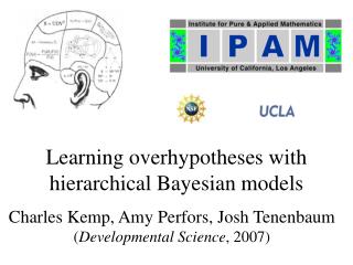
Structure and statistics • A framework for understanding how structured knowledge and statistical inference interact. • How structured knowledge guides statistical inference, and is itself acquired through higher-order statistical learning. Hierarchical Bayes. • How simplicity trades off with fit to the data in evaluating structural hypotheses. Bayesian Occam’s Razor. • How increasingly complex structures may grow as required by new data, rather than being pre-specified in advance. Non-parametric Bayes.
Alternative approaches to inductive generalization • Associative learning • Connectionist networks • Similarity to examples • Toolkit of simple heuristics • Constraint satisfaction • Analogical mapping
Marr’s Three Levels of Analysis • Computation: “What is the goal of the computation, why is it appropriate, and what is the logic of the strategy by which it can be carried out?” • Representation and algorithm: Cognitive psychology • Implementation: Neurobiology
Why Bayes? • A framework for explaining cognition. • How people can learn so much from such limited data. • Why process-level models work the way that they do. • Strong quantitative models with minimal ad hoc assumptions. • A framework for understanding how structured knowledge and statistical inference interact. • How structured knowledge guides statistical inference, and is itself acquired through higher-order statistical learning. • How simplicity trades off with fit to the data in evaluating structural hypotheses (Occam’s razor). • How increasingly complex structures may grow as required by new data, rather than being pre-specified in advance.
Outline • Morning • Introduction (Josh) • Basic case study #1: Flipping coins (Tom) • Basic case study #2: Rules and similarity (Josh) • Afternoon • Advanced case study #1: Causal induction (Tom) • Advanced case study #2: Property induction (Josh) • Quick tour of more advanced topics (Tom)
Coin flipping HHTHT HHHHH What process produced these sequences?
Bayes’ rule • “Posterior probability”: • “Prior probability”: • “Likelihood”: For data D and a hypothesis H, we have:
The origin of Bayes’ rule • A simple consequence of using probability to represent degrees of belief • For any two random variables:
Why represent degrees of belief with probabilities? • Good statistics • consistency, and worst-case error bounds. • Cox Axioms • necessary to cohere with common sense • “Dutch Book” + Survival of the Fittest • if your beliefs do not accord with the laws of probability, then you can always be out-gambled by someone whose beliefs do so accord. • Provides a theory of learning • a common currency for combining prior knowledge and the lessons of experience.
Bayes’ rule • “Posterior probability”: • “Prior probability”: • “Likelihood”: For data D and a hypothesis H, we have:
Hypotheses in Bayesian inference • Hypotheses H refer to processes that could have generated the data D • Bayesian inference provides a distribution over these hypotheses, given D • P(D|H) is the probability of D being generated by the process identified by H • Hypotheses H are mutually exclusive: only one process could have generated D
statistical models Hypotheses in coin flipping Describe processes by which D could be generated • Fair coin, P(H) = 0.5 • Coin with P(H) = p • Markov model • Hidden Markov model • ... D = HHTHT
generative models Hypotheses in coin flipping Describe processes by which D could be generated • Fair coin, P(H) = 0.5 • Coin with P(H) = p • Markov model • Hidden Markov model • ... D = HHTHT
Graphical model notation Pearl (1988), Jordan (1998) Variables are nodes, edges indicate dependency Directed edges show causal process of data generation d1d2 d3 d4 Fair coin, P(H) = 0.5 d1d2 d3 d4 Markov model HHTHT d1d2 d3 d4 d5 Representing generative models
p d1d2 d3 d4 P(H) = p s1s2 s3 s4 HHTHT d1d2 d3 d4 Hidden Markov model d1d2 d3 d4 d5 Models with latent structure • Not all nodes in a graphical model need to be observed • Some variables reflect latent structure, used in generating D but unobserved
Coin flipping • Comparing two simple hypotheses • P(H) = 0.5 vs. P(H) = 1.0 • Comparing simple and complex hypotheses • P(H) = 0.5 vs. P(H) = p • Comparing infinitely many hypotheses • P(H) = p • Psychology: Representativeness
Coin flipping • Comparing two simple hypotheses • P(H) = 0.5 vs. P(H) = 1.0 • Comparing simple and complex hypotheses • P(H) = 0.5 vs. P(H) = p • Comparing infinitely many hypotheses • P(H) = p • Psychology: Representativeness
Comparing two simple hypotheses • Contrast simple hypotheses: • H1: “fair coin”, P(H) = 0.5 • H2:“always heads”, P(H) = 1.0 • Bayes’ rule: • With two hypotheses, use odds form
Bayes’ rule in odds form = x P(H1|D) P(D|H1) P(H1) P(H2|D) P(D|H2) P(H2) D: data H1, H2: models P(H1|D): posterior probability H1 generated the data P(D|H1): likelihood of data under model H1 P(H1): prior probability H1 generated the data
Coin flipping HHTHT HHHHH What process produced these sequences?
Comparing two simple hypotheses = x P(H1|D) P(D|H1) P(H1) P(H2|D) P(D|H2) P(H2) D: HHTHT H1, H2: “fair coin”, “always heads” P(D|H1) = 1/25P(H1) = 999/1000 P(D|H2) = 0 P(H2) = 1/1000 P(H1|D) / P(H2|D) = infinity
Comparing two simple hypotheses = x P(H1|D) P(D|H1) P(H1) P(H2|D) P(D|H2) P(H2) D: HHHHH H1, H2: “fair coin”, “always heads” P(D|H1) = 1/25 P(H1) = 999/1000 P(D|H2) = 1 P(H2) = 1/1000 P(H1|D) / P(H2|D) 30
Comparing two simple hypotheses = x P(H1|D) P(D|H1) P(H1) P(H2|D) P(D|H2) P(H2) D: HHHHHHHHHH H1, H2: “fair coin”, “always heads” P(D|H1) = 1/210 P(H1) = 999/1000 P(D|H2) = 1P(H2) = 1/1000 P(H1|D) / P(H2|D) 1
Comparing two simple hypotheses • Bayes’ rule tells us how to combine prior beliefs with new data • top-down and bottom-up influences • As a model of human inference • predicts conclusions drawn from data • identifies point at which prior beliefs are overwhelmed by new experiences • But… more complex cases?
Coin flipping • Comparing two simple hypotheses • P(H) = 0.5 vs. P(H) = 1.0 • Comparing simple and complex hypotheses • P(H) = 0.5 vs. P(H) = p • Comparing infinitely many hypotheses • P(H) = p • Psychology: Representativeness
p d1d2 d3 d4 d1d2 d3 d4 Fair coin, P(H) = 0.5 P(H) = p Comparing simple and complex hypotheses • Which provides a better account of the data: the simple hypothesis of a fair coin, or the complex hypothesis that P(H) = p? vs.
Comparing simple and complex hypotheses • P(H) = p is more complex than P(H) = 0.5 in two ways: • P(H) = 0.5 is a special case of P(H) = p • for any observed sequence X, we can choose p such that X is more probable than if P(H) = 0.5
Comparing simple and complex hypotheses Probability
Comparing simple and complex hypotheses Probability HHHHH p = 1.0
Comparing simple and complex hypotheses Probability HHTHT p = 0.6
Comparing simple and complex hypotheses • P(H) = p is more complex than P(H) = 0.5 in two ways: • P(H) = 0.5 is a special case of P(H) = p • for any observed sequence X, we can choose p such that X is more probable than if P(H) = 0.5 • How can we deal with this? • frequentist: hypothesis testing • information theorist: minimum description length • Bayesian: just use probability theory!
Comparing simple and complex hypotheses P(H1|D) P(D|H1) P(H1) P(H2|D) P(D|H2) P(H2) Computing P(D|H1) is easy: P(D|H1) = 1/2N Compute P(D|H2) by averaging over p: = x
Comparing simple and complex hypotheses Probability Distribution is an average over all values of p