Bayesian Learning
Bayesian Learning. Evgueni Smirnov. Overview. Bayesian Theorem Maximum A Posteriori Hypothesis Naïve Bayes Classifier Learning Text Classifiers. Thomas Bayes (1702- 1761).


Bayesian Learning
E N D
Presentation Transcript
Bayesian Learning Evgueni Smirnov
Overview • Bayesian Theorem • Maximum A Posteriori Hypothesis • Naïve Bayes Classifier • Learning Text Classifiers
Thomas Bayes (1702- 1761) Bayesian theory of probability was set out in 1764. His conclusions were accepted by Laplace in 1781, rediscovered by Condorcet, and remained unchallenged until Boole questioned them.
Bayes Theorem Goal: To determine the posterior probability of hypothesis h given the data D from: • Prior probability of h, P(h): it reflects any background knowledge we have about the chance that h is a correct hypothesis (before having observed the data). • Prior probability of D, P(D): it reflects the probability that training data D will be observed given no knowledge about which hypothesis h holds. • Conditional Probability of observation D, P(D|h): it denotes the probability of observing data D given some world in which hypothesis h holds.
Bayes Theorem • Posterior probability of h, P(h|D): it represents the probability that h holds given the observed training data D. It reflects our confidence that h holds after we have seen the training data D and it is the quantity that Data-mining researchers are interested in. • Bayes Theorem allows us to compute P(h|D):
Maximum a Posteriori Hypothesis (MAP) In many learning scenarios, the learner considers a set of hypotheses H and is interested in finding the most probable hypothesis h H given the observed data D. Any such hypothesis is called maximum a posteriori hypothesis.
Example Consider a cancer test with two outcomes: positive [+] and negative [-]. The test returns a correct positive result in 98% of the cases in which the disease is actually present, and a correct negative result in 97% of the cases in which the disease is not present. Furthermore, .008 of all people have this cancer. P(cancer) = 0.008 P(cancer) = 0.992 P([+] | cancer) = 0.98 P([-] | cancer) = 0.02 P([+] | cancer) = 0.03 P([-] | cancer) = 0.97 A patient got a positive test [+]. The maximum a posteriori hypothesis is: P([+] | cancer)P(cancer) = 0.98 x 0.008 = 0.0078 P([+] | cancer)P( cancer) = 0.03 x 0.992 = 0.0298 hMAP= cancer
Naïve Bayes Classifier Let each instance x of a training set D be described by a conjunction of n attribute values < a1(x), a2(x), … an(x) > and we have a finite set V of possible classes (concepts). Naïve Bayes assumption is that attributes are conditionally independent!
Example Consider the weather data and we have to classify the instance: < Outlook = sunny, Temp = cool, Hum = high, Wind = strong> The task is to predict the value (yes or no) of the concept PlayTennis. We apply the naïve bayes rule:
Example Thus, the naïve Bayes classifier assigns the value no to PlayTennis!
Estimating Probabilities • To estimate the probability P(ai(x) | vj) we use: • Relative frequency: nc/n, where nc is the number of training instances that belong to the class vjand have value ai(x) for the attribute ai, and n is the number of training instances of the class vj; • m-estimate: (nc+ mp)/(n+m), where nc is the number of training instances that belong to the class vjand have value ai(x) for the attribute ai, n is the number of training instances of the class vj, p is the prior estimate of the probablity of the class P(ai(x) | vj) , and m is the weight of P(ai(x) | vj) .
Learning to Classify Text • Simplifications: • each document is represented by a vector of words; • the words are considered as numerical attributes wk; • the values of the word attributes wk are the frequencies the words occur in the text. • To estimate the probability P(wk | v) we use: • where n is the total number of word positions in all the documents (instances) whose target value is v, nk is the number of times word wk is found in these n word positions, and |Vocabulary| is the total number of distinct words found in the training data.
Summary • Bayesian methods provide the basis for probabilistic learning methods that use knowledge about the prior probabilities of hypotheses and about the probability of observing data given the hypothesis; • Bayesian methods can be used to determine the most probable hypothesis given the data; • The naive Bayes classifier is useful in many practical applications.