Bayesian Learning
Bayesian Learning. Bayesian Learning. Probabilistic approach to inference Assumption Quantities of interest are governed by probability distribution Optimal decisions can be made by reasoning about probabilities and observations

Bayesian Learning
E N D
Presentation Transcript
Bayesian Learning Computer Science Department CS 9633 Machine Learning
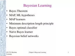
Bayesian Learning • Probabilistic approach to inference • Assumption • Quantities of interest are governed by probability distribution • Optimal decisions can be made by reasoning about probabilities and observations • Provides quantitative approach to weighing how evidence supports alternative hypotheses Computer Science Department CS 9633 Machine Learning
Why is Bayesian Learning Important? • Some Bayesian approaches (like naive Bayes) are very practical learning approaches and competitive with other approaches • Provides a useful perspective for understanding many learning algorithms that do not explicitly manipulate probabilities Computer Science Department CS 9633 Machine Learning
Important Features • Model is incrementally updated with training examples • Prior knowledge can be combined with observed data to determine the final probability of the hypothesis • Asserting prior probability of candidate hypotheses • Asserting a probability distribution over observations for each hypothesis • Can accommodate methods that make probabilistic predictions • New instances can be classified by combining predictions of multiple hypotheses • Can provide a gold standard for evaluating hypotheses Computer Science Department CS 9633 Machine Learning
Practical Problems • Typically require initial knowledge of many probabilities. Can be estimated by: • Background knowledge • Previously available data • Assumptions about distribution • Significant computational cost of determining Bayes optimal hypothesis in general • linear in number of hypotheses in general case • Significantly lower for certain situations Computer Science Department CS 9633 Machine Learning
Bayes Theorem • Goal: learn the “best” hypothesis • Assumption in Bayes learning: the “best” hypothesis is the most probable hypothesis • Bayes theorem allows computation of most probable hypothesis based on • Prior probability of hypothesis • Probability of observing certain data given the hypothesis • Observed data itself Computer Science Department CS 9633 Machine Learning
Notation P(h) Prior probability of h P(D) Prior probability of D P(D|h) Probability of D given h posterior probability of D given h likelihood of Data given h P(h|D) Probability that h holds, given the data Computer Science Department CS 9633 Machine Learning
Bayes Theorem • Based on definitions of P(D|h) and P(h|D) D h Computer Science Department CS 9633 Machine Learning
Maximum A Posteriori Hypothesis • Many learning algorithms try to identify the most probable hypothesis h H given observations D • This is the maximum a posteriori hypothesis (MAP hypothesis) Computer Science Department CS 9633 Machine Learning
Identifying the MAP Hypothesis using Bayes Theorem Computer Science Department CS 9633 Machine Learning
Equally Probable Hypotheses Any hypothesis that maximizes P(D|h) is a Maximum Likelihood (ML) hypothesis Computer Science Department CS 9633 Machine Learning
Bayes Theorem and Concept Learning • Concept Learning Task H Hypothesis space X Instance space c: X{0,1} Computer Science Department CS 9633 Machine Learning
Brute-Force MAP Learning Algorithm • For each hypothesis h in H, calculate the posterior probability • Output the hypothesis with the highest posterior probability Computer Science Department CS 9633 Machine Learning
To Apply Brute Force MAP Learning • Specify P(h) • Specify P(D|h) Computer Science Department CS 9633 Machine Learning
An Example • Assume • Training data D is noise free (di = c(xi)) • The target concept is contained in H • We have no a priori reason to believe one hypothesis is more likely than any other Computer Science Department CS 9633 Machine Learning
Probability of Data Given Hypothesis Computer Science Department CS 9633 Machine Learning
Apply the algorithm • Step 1 (2 cases) • Case 1 (D is inconsistent with h) • Case 2 (D is consistent with h) Computer Science Department CS 9633 Machine Learning
Step 2 • Every consistent hypothesis has probability 1/|VSH,D| • Every inconsistent hypothesis has probability 0 Computer Science Department CS 9633 Machine Learning
MAP hypothesis and consistent learners • FIND-S (finds maximally specific consistent hypothesis) • Candidate-Elimination (finds all consistent hypotheses. Computer Science Department CS 9633 Machine Learning
Maximum Likelihood and Least-Squared Error Learning • New problem: learning a continuous-valued target function • Will show that under certain assumptions, any learning algorithm that minimized the squared error between output hypotheses on training data will output a maximum likelihood hypothesis. Computer Science Department CS 9633 Machine Learning
Problem Setting • Learner L • Instance space X • Hypothesis space H h: XR • Task of L is to learn unknown target function f: XR • Have m examples • Target value for each example is corrupted by random noise drawn from Normal distribution Computer Science Department CS 9633 Machine Learning
Work Through Derivation Computer Science Department CS 9633 Machine Learning
Why Normal Distribution for Noise? • Its easy to work with • Good approximation of many physical processes • Important point: we are only dealing with noise in the target function—not the attribute values. Computer Science Department CS 9633 Machine Learning
Bayes Optimal Classifier • Two Questions: • What is the most probable hypothesis given the training data? • Find MAP hypothesis • What is the most probable classification given the training data? Computer Science Department CS 9633 Machine Learning
Example • Three hypotheses: P(h1|D) = 0.35 P(h2|D) = 0.45 P(h3|D) = 0.20 • New instance x h1 predicts negative h2 predicts positive h3 predicts negative • What is the predicted class using hMAP? • What is the predicted class using all hypotheses? Computer Science Department CS 9633 Machine Learning
Bayes Optimal Classification • The most probable classification of a new instance is obtained by combining the predictions of all hypotheses, weighted by their posterior probabilities. • Suppose set of values for classification is from set V (each possible value is vj) • Probability that vj is the correct classification for new instance is: • Pick the vj with the max probability as the predicted class Computer Science Department CS 9633 Machine Learning
Bayes Optimal Classifier Apply this to the previous example: Computer Science Department CS 9633 Machine Learning
Bayes Optimal Classification • Gives the optimal error-minimizing solution to prediction and classification problems. • Requires probability of exact combination of evidence • All classification methods can be viewed as approximations of Bayes rule with varying assumptions about conditional probabilities • Assume they come from some distribution • Assume conditional independence • Assume underlying model of specific format (linear combination of evidence, decision tree) Computer Science Department CS 9633 Machine Learning
Simplifications of Bayes Rule • Given observations of attribute values a1, a2, …an,, compute the most probable target value vMAP • Use Bayes Theorem to rewrite Computer Science Department CS 9633 Machine Learning
Naïve Bayes • The most usual simplification of Bayes Rule is to assume conditional independence of the observations • Because it is approximately true • Because it is computationally convenient • Assume the probability of observing the conjunction a1, a2, …an is the product of the probabilities of the individual attributes • Learning consists of estimating probabilities Computer Science Department CS 9633 Machine Learning
Simple Example • Two classes C1 and C2. • Two features • a1 Male, Female • a2 Blue eyes, Brown eyes • Instance (Male with blue eyes) What is the class? Computer Science Department CS 9633 Machine Learning
Estimating Probabilities(Classifying Executables) • Two Classes (Malicious, Benign) • Features • a1 GUI present (yes/no) • a2 Deletes files (yes/no) • a3 Allocates memory (yes/no) • a4 Length (< 1K, 1-10 K, > 10K) Computer Science Department CS 9633 Machine Learning
Classify the Following Instance • <Yes, No, Yes, Yes> Computer Science Department CS 9633 Machine Learning
Estimating Probabilities • To estimate P(C|D) • Let n be the number of training examples labeled D • Let nc be the number labeled D that are also labeled C • P(C|D) was estimated as nc/n • Problems • This is a biased underestimate of the probability • When the term is 0, it dominates all others Computer Science Department CS 9633 Machine Learning
Use m-estimate of probability • p is prior of what we are trying to estimate (often assume attribute values equally probable) • m is a constant (called equivalent sample size) view this augmenting with a virtual sample Computer Science Department CS 9633 Machine Learning
Repeat Estimates • Use equal priors for attribute values • Use m value of 1 Computer Science Department CS 9633 Machine Learning
Bayesian Belief Networks • Naïve Bayes is based on assumption of conditional independence • Bayesian networks provide a tractable method for specifying dependencies among variables Computer Science Department CS 9633 Machine Learning
Terminology • A Bayesian Belief Network describes the probability distribution over a set of random variables Y1, Y2, …Yn • Each variable Yi can take on the set of values V(Yi) • The joint space of the set of variables Y is the cross product V(Y1) V(Y2) … V(Yn) • Each item in the joint space corresponds to one possible assignment of values to the tuple of variables <Y1, …Yn> • Joint probability distribution: specifies the probabilities of the items in the joint space • A Bayesian Network provides a way to describe the joint probability distribution in a compact manner. Computer Science Department CS 9633 Machine Learning
Conditional Independence • Let X, Y, and Z be three discrete-valued random variables. • We say that X is conditionally independent of Y given Z if the probability distribution governing X is independent of the value of Y given a value for Z Computer Science Department CS 9633 Machine Learning
Bayesian Belief Network • A set of random variables makes up the nodes of the network • A set of directed links or arrows connects pairs of nodes. The intuitive meaning of an arrow from X to Y is that X has a direct influence on Y. • Each node has a conditional probability table that quantifies the effects that the parents have on the node. The parents of a node are all those nodes that have arrows pointing to it. • The graph has no directed cycles (it is a DAG) Computer Science Department CS 9633 Machine Learning
Example (from Judea Pearl) You have a new burglar alarm installed at home. It is fairly reliable at detecting a burglary, but also responds on occasion to minor earthquakes. You also have two neighbors, John and Mary, who have promised to call you at work when they hear the alarm. John always calls when he hears the alarm, but sometimes confuses the telephone ringing with the alarm and calls then, too. Mary, on the other hand, likes rather loud music and sometimes misses the alarm altogether. Given the evidence of who has or has not called, we would like to estimate the probability of a burglary. Computer Science Department CS 9633 Machine Learning
Step 1 • Determine what the propositional (random) variables should be • Determine causal (or another type of influence) relationships and develop the topology of the network Computer Science Department CS 9633 Machine Learning
Topology of Belief Network Burglary Earthquake Alarm JohnCalls MaryCalls Computer Science Department CS 9633 Machine Learning
Step 2 • Specify a conditional probability table or CPT for each node. • Each row in the table contains the conditional probability of each node value for a conditioning case (possible combinations of values for parent nodes). • In the example, the possible values for each node are true/false. • The sum of the probabilities for each value of a node given a particular conditioning case is 1. Computer Science Department CS 9633 Machine Learning
Example:CPT for Alarm Node P(Alarm|Burglary,Earthquake) TrueFalse Earthquake Burglary True True 0.950 0.050 True False 0.940 0.060 False True 0.290 0.710 False False 0.001 0.999 Computer Science Department CS 9633 Machine Learning
Complete Belief Network P(B) 0.001 P(E) 0.002 Burglary Earthquake B E P(A|B,E) T T 0.95 T F 0.94 F T 0.29 F F 0.01 Alarm A P(J|A) T 0.90 F 0.05 A P(M|A) T 0.70 F 0.01 JohnCalls MaryCalls Computer Science Department CS 9633 Machine Learning
Semantics of Belief Networks • View 1: A belief network is a representation of the joint probability distribution (“joint”) of a domain. • The joint completely specifies an agent’s probability assignments to all propositions in the domain (both simple and complex.) Computer Science Department CS 9633 Machine Learning
Network as representation of joint • A generic entry in the joint probability distribution is the probability of a conjunction of particular assignments to each variable, such as: • Each entry in the joint is represented by the product of appropriate elements of the CPTs in the belief network. Computer Science Department CS 9633 Machine Learning
Example Calculation Calculate the probability of the event that the alarm has sounded but neither a burglary nor an earthquake has occurred, and both John and Mary call. P(J ^ M ^ A ^ ~B ^ ~E) = P(J|A) P(M|A) P(A|~B,~E) P(~B) P(~E) = 0.90 * 0.70 * 0.001 * 0.999 * 0.998 = 0.00062 Computer Science Department CS 9633 Machine Learning

