Bayesian Learning
Explore how Bayesian learning algorithms calculate explicit probabilities, with a focus on the influential Naïve Bayes classifier. Bayesian methods can analyze diverse algorithms, accommodating probabilistic predictions for optimal decision making. Discover the practical difficulties associated with Bayesian learning and explore key theorems like Bayes' Theorem. Learn about optimal codes and the concept of minimal description length.

Bayesian Learning
E N D
Presentation Transcript
Bayesian Learning Computer Science 760 Patricia J Riddle 760 bayes & hmm
Introduction Bayesian learning algorithms calculate explicit probabilities for hypotheses Naïve Bayes classifier is among the most effective in classifying text documents Bayesian methods can also be used to analyze other algorithms Training example incrementally increases or decreases the estimated probability that a hypothesis is correct Prior knowledge can be combined with observed data to determine the final probability of a hypothesis 760 bayes & hmm
Prior Knowledge Prior knowledge is: • Prior probability for each candidate hypothesis and • A probability distribution over observed data 760 bayes & hmm
Bayesian Methods in Practice Bayesian methods accommodate hypotheses that make probabilistic predictions “this pneumonia patient has a 98% chance of complete recovery” New instances can be classified by combining the predictions of multiple hypotheses, weighted by their probabilities Even when computationally intractable, they can provide a standard of optimal decision making against which other practical measures can be measured 760 bayes & hmm
Practical Difficulties • Require initial knowledge of many probabilities - estimated based on background knowledge, previously available data, assumptions about the form of the underlying distributions • Significant computational cost to determine the Bayes optimal hypothesis in the general case - linear in the number of candidate hypotheses - in certain specialized situations the cost can be significantly reduced 760 bayes & hmm
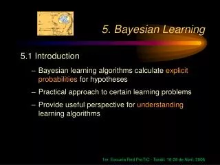
Bayes Theorem Intuition Learning - we want the best hypothesis from some space H, given the observed training data D. Best can be defined as most probable given the data D plus any initial knowledge about prior probabilities of the various hypotheses in H. This is a direct method!!! (No Search) 760 bayes & hmm
Bayes Terminology P(h) – the prior probability that hypothesis h holds before we observe the training data - prior probability - if we have no prior knowledge we assign the same initial probability to them all (it is trickier than this!!) P(D) - prior probability training data D will be observed given no knowledge about which hypothesis holds P(D|h) - the probability of observing data D given that hypothesis h holds P(h|D) - the probability that h holds given the training data D - posterior probability 760 bayes & hmm
Bayes Theorem Probability increases with P(h) and P(D|h) and decreases with P(D) - this last is not true with a lot of other scoring functions! 760 bayes & hmm
MAP & ML Hypothesis So we want a maximum a posteriori hypothesis (MAP) - P(D) same for every hypothesis If we assume every hypothesis is equally likely a priori then we want the maximum likelihood hypothesis Bayes theorem is more general than Machine Learning!! 760 bayes & hmm
A general Example Two hypothesis: the patient has cancer, , the patient doesn’t have cancer, Prior knowledge: over the entire population of people .008 have cancer The lab test returns a correct positive result in 98% of the cases in which cancer is actually present and a correct negative in 97% of the cases in which cancer is actually not present P(cancer) = .008, P(¬cancer) = .992 P(|cancer) = .98, P(|cancer) = .02 P(|¬cancer)=.03, P(|¬cancer)=.97 So given a new patient with a positive lab test, should we diagnose the patient as having cancer or not?? Which is the MAP hypothesis? 760 bayes & hmm
Example Answer Has cancer - P(|cancer)P(cancer) = (.98).008 = .0078 Doesn’t have cancer - P(|¬cancer)P(¬cancer)=(.03).992=.0298 hMAP=¬cancer Exact posterior probabilities – Posterior as a real probability 760 bayes & hmm
Minimum Description Length Let us look at hMAP in the light of basic concepts of information theory hMAP argmaxhH P(D|h) P(h) = argminhH - log2P(D|h) - log2P(h) This can be interpreted as a statement that short hypotheses are preferred. 760 bayes & hmm
Information Theory • Consider the problem of designing a code to transmit messages drawn at random, where the probability of encountering message i is pi. • We want the code that minimizes the expected number of bits we must transmit in order to encode a message drawn at random. • To minimize the expected code length we should assign shorter codes to more probable messages. 760 bayes & hmm
Optimal Code • Shannon and Weaver (1949) showed the optimal code assigns -log2pi bits to encode message i. Where pi is the probability of i appearing. • LC(i) is the description length of message i with respect to code C. • LCH is the size of the description of the hypothesis h using the optimal representation for encoding the hypothesis space H. • LCD|h is the size of the description of the training data D given the hypothesis h using the optimal representation for encoding the data D assuming that both the sender and receiver know the hypothesis h. 760 bayes & hmm
Applying MDL • To apply this principle we must choose specific representations C1 and C2 appropriate for the given learning task! • Minimum Description Length Principle: • If C1 and C2 are chosen to be optimal encodings for their respective tasks, then hMDL=hMAP 760 bayes & hmm
MDL Example • Apply MDL principle to the problem of learning decision trees. • C1 is an encoding of trees where the description length grows with the number of nodes in the tree and the number of edges. • C2 transmits misclassified examples by identifying • which example is misclassified (log2m bits, where m is the number of training instances) and • its correct classification (log2k bits, where k is the number of classes). 760 bayes & hmm
MDL Intuition MDL principle provides a way of trading off hypothesis complexity for the number of errors committed by the hypothesis So the MDL principle produces a MAP hypothesis if the encodings C1 and C2 are optimal. But to show that we would need all the prior probabilities P(h) as well as P(D|h). No reason to believe the MDL hypothesis relative to arbitrary encodings should be preferred!!!! 760 bayes & hmm
What I hate about MDL “But you did’t find the optimal encodings C1 and C2.” “Well it doesn’t matter if you see enough data it doesn’t matter which one you use.” So why are we using a Bayesian approach???? 760 bayes & hmm
Bayes Optimal Classifier What is the most probable classification of the new instance given the training data? Could just apply the MAP hypothesis, but can do better!!! 760 bayes & hmm
Bayes Optimal Intuitions Assume three hypothesis h1, h2, h3 whose posterior probabilities are .4, .3 and .3 respectively. Thus h1 is the MAP hypothesis. Suppose we have a new instance x which is classified positive by h1 and negative by h2 and h3. Taking all hypothesis into account, the probability that x is positive is .4 and the probability it is negative is .6. The most probable classification (negative) is different than the classification given by the MAP hypothesis!!! 760 bayes & hmm
Bayes Optimal Classifier II We want to combine the predictions of all hypotheses weighted by their posterior probabilities. where vj is from the set of classifications V. Bayes Optimal Classification: No other learner using the same hypothesis space and same prior knowledgecan outperform this method on average. It maximizes the probability that the new instance is classified correctly. 760 bayes & hmm
Gibbs Algorithm Bayes Optimal is quite costly to apply. It computes the posterior probabilities for every hypothesis in H and combines the predictions of each hypothesis to classify each new instance. An alternative (less optimal) method: • Choose a hypothesis h from H at random, according to the posterior probability distribution over H. • Use h to predict the classification of the next instance x. Under certain conditions the expected misclassification error for Gibbs algorithm is at most twice the expected error of the Bayes optimal classifier. 760 bayes & hmm
What is Naïve Bayes? Results comparable to ANN and decision trees in some domains Each instance x is described by a conjunction of attribute values and the target value f(x) can take any value from a set V. A set of training instances are provided and a new instance is presented and the learner is asked to predict the target value. P(vj) is estimated by the frequency of each target value in the training data. Cannot use frequency for P(a1,a2,…an|vj) unless we have a very, very large set of training data to get a reliable estimate. 760 bayes & hmm
Conditional Independence Naïve Bayes assumes attribute values are conditionally independently given the target value - Naïve Bayes Classifier: where vNB denotes the target values P(ai|vj) can be estimated by frequency 760 bayes & hmm
When is Naïve Bayes a MAP? When conditional independence assumption is satisfied the naïve Bayes classification is a MAP classification Naïve Bayes entails no search!! 760 bayes & hmm
An Example Target concept PlayTennis Classify the following instance: <Outlook=sunny, Temperature = cool, Humidity = high, Wind = strong> P(PlayTennis=yes)=9/14=.64 P(PlayTennis=no)=5/14=.36 P(Wind=strong|PlayTennis=yes)=3/9=.33 P(Wind=strong|PlayTennis=no)=3/5=.60 ….. 760 bayes & hmm
An Example II P(yes) P(sunny|yes) P(cool|yes) P(high|yes) P(strong|yes) = .0053 P(no) P(sunny|no) P(cool|no) P(high|no) P(strong|no) = .0206 Naïve Bayes returns “Play Tennis = no” with probability 760 bayes & hmm
Naïve Bayes used for Document Clustering • Are the words conditionally independent? • Works really well anyway 760 bayes & hmm
Bayesian Belief Networks • Naïve Bayes assumes all the attributes are conditionally independent • Bayesian Belief Networks (BBNs) describe a joint probability distribution over a set of variables by specifying a set of conditional independence assumptions and a set of conditional probabilities • X is conditionally independent of Y means P(X|Y,Z) = P(X|Z) 760 bayes & hmm
A Bayesian Belief Network Storm BusTourGroup S,B S,¬B ¬S,B ¬S,¬B C 0.4 0.1 0.8 0.2 ¬C 0.6 0.9 0.2 0.8 Lightning Campfire Campfire Thunder ForestFire 760 bayes & hmm
Representation • Each variable is represented by a node and has two types of information specified. • Arcs representing the assertions that the variable is conditionally independent of its nondescendents given its immediate predecessors (I.e., Parents). X is a descendent of Y if there is a directed path from Y to X. • A conditional probability table describing the probability distribution for that variable given the values of its immediate predecessors. This joint probability is computed by 760 bayes & hmm
Representation II • Campfire is conditionally independent of its nondescendents Lightning and Thunder given its parents Storm and BusTourGroup • Also notice that ForestFire is conditionally independent of BusTourGroup and Thunder given Campfire and Storm and Lightning. • Similarly, Thunder is conditionally independent of Storm, BusTourGroup, Campfire, and ForestFire given Lightning. • BBNs are a convenient way to represent causal knowledge. The fact that Lightning causes Thunder is represented in the BBN by the fact that Thunder is conditionally independent of other variables in the network given the value of Lightning. 760 bayes & hmm
Inference • Can we use the BBN to infer the value of a target variable ForestFire given the observed values of the other variables. • Infer not a single value but the probability distribution for the target variable which specifies the probability it will take on each possible value given the observed values of the other variables • Generally, we may wish to infer the probability distribution of a variable (e.g., ForestFire) given observed values for only a subset of the other variables (e.g., Thunder and BusTourGroup are the only observed values available). • Exact inference of probabilities (and even some approximate methods) for an arbitrary BBN is known to be NP-hard. • Monte Carlo methods provide approximate solutions by randomly sampling the distributions of the unobserved variables 760 bayes & hmm
Learning BBNs • If the network structure was given in advance and the variables are fully observable, then just use the Naïve Bayes formula modulo only some of the variables are conditionally independent. • If the network structure is given but only some of the variables are observable, the problem is analogous to learning weights for the hidden units in an ANN. • Similarly, use a gradient ascent procedure to search through the space of hypotheses that corresponds to all possible entries in the conditional probability tables. The objective function that is maximized is P(D|h). • By definition this corresponds to searching for the maximum likelihood hypothesis for the table entries. 760 bayes & hmm
Gradient Ascent Training of BBN • Let wijk denote a single entry in one of the conditional probability tables. Specifically that variable Yi will take on value yij given that its parents Ui take on the values uik. • If wijk is the top right entry, then Yi is the variable Campfire, Ui is the tuple of parents <Storm, BusTourGroup>, yij=True and uik=<False,False>. • The derivative for each wijk is 760 bayes & hmm
Weight Updates • So back to our example we must calculate P(Campfire = True, Storm = False, BusTourGroup = False | d) for each training example d in D. If the required probability is unobservable then we can calculate it from other variables using standard BBN inference. • As weights wijk are updated they must remain in the interval [0,1] and the sum j wijk remains 1 for all i,k. So must have a two step process. • Renormalize the weights wijk • Will converge to a locally maximum likelihood hypothesis for the conditional probabilities in the BBn. 760 bayes & hmm
Summary • Bayesian methods provide a basis for probabilistic learning methods that accommodate knowledge about prior distributions of alternative hypothesis and about the probability of observing the data given various hypothesis. They assign a posterior probability to each candidate hypothesis, based on these assumed priors and the observed data, • Bayesian methods return the most probable hypothesis (e.g., a MAP hypothesis). • Bayes Optimal classfier combines the predictions of all alternative hypotheses weighted by their posterior probabilities, to calculate the most probable classification of a new instance. 760 bayes & hmm
Naïve Bayes Summary • Naïve Bayes has been found to be useful in many killer apps. • It is naïve because it has no street sense….no no no…it incorporates the simplifying assumption that attribute values are conditionally independent given the classification of the instance. • When this is true naïve Bayes produces a MAP hypothesis. • Even when the assumption is violated Naïve Bayes tends to perform well. • BBNs provide a more expressive representation for sets of conditional independence assumptions. 760 bayes & hmm
Minimum Description Length Summary • The Minimum Description Length principle recommends choosing the hypothesis that minimizes the description length of the hypothesis plus the description length of the data given the hypothesis. • Bayes theorem and basic results from information theory can be used to provide a rationale for this principle. 760 bayes & hmm
Hidden Markov Models Comp Sci 369 Dr Patricia Riddle 760 bayes & hmm
Automata Theory An automaton is a mathematical model for a finite state machine (FSM). An FSM is a machine that, given an input of symbols, 'jumps' through a series of states according to a transition function (which can be expressed as a table). 760 bayes & hmm
Finite State Machine A model of computation consisting of a set of states, a start state, an input alphabet, and a transition functionthat maps input symbols and current states to a next state. Computation begins in the start state with an input string. It changes to new states depending on the transition function. Also known as finite state automaton 760 bayes & hmm
Transition 760 bayes & hmm
Deterministic Finite Automata 760 bayes & hmm
Nondeterministic Finite Automata 760 bayes & hmm
Variations There are many variants, for instance, machines having actions (outputs) associated with transitions (Mealy machine) or states (Moore machine), multiple start states, transitions conditioned on no input symbol (a null) more than one transition for a given symbol and state (nondeterministic finite state machine), one or more states designated as accepting states (recognizer), etc. 760 bayes & hmm
Finite State Machines An automaton is represented by the 5-tuple <Q,,,q0,F>, where: Q is a set of states. • is a finite set of symbols, that we will call the alphabet of the language the automaton accepts. • is the transition function, that is : QxQ (For non-deterministic automata, the empty string is an allowed input). q0 is the start state, that is, the state in which the automaton is when no input has been processed yet (Obviously, q0∈ Q). F is a set of states of Q (i.e. F⊆Q), called accept states. 760 bayes & hmm
Markov Chains - CS Definition Markov chain - A finite state machinewith probabilities for each transition, that is, a probability that the next state is sj given that the current state is si. Note: Equivalently, a weighted, directed graphin which the weights correspond to the probability of that transition. In other words, the weights are nonnegative and the total weight of outgoing edges is positive. If the weights are normalized, the total weight, including self-loops, is 1. 760 bayes & hmm
Markov Chain Graph 760 bayes & hmm
Markov Chain Example 760 bayes & hmm