A Regression Model for Ensemble Forecasts
A Regression Model for Ensemble Forecasts. David Unger Climate Prediction Center. Summary. A linear regression model can be designed specifically for ensemble prediction systems. It is best applied to direct model forecasts of the element in question.

A Regression Model for Ensemble Forecasts
E N D
Presentation Transcript
A Regression Model for Ensemble Forecasts David Unger Climate Prediction Center
Summary • A linear regression model can be designed specifically for ensemble prediction systems. • It is best applied to direct model forecasts of the element in question. • Ensemble regression is easy to implement and calibrate. • This talk will summarize how it works
Ensemble Forecasting The ensemble forecasting approach is based on the following beliefs: 1) Individual solutions represent possible outcomes. 2) Each ensemble member is equally likely to best represent the observation. 3) The ensemble set behaves as a randomly selected sample from the expected distribution of observations.
A Schematic Drawing of an Ensemble Regression Line. Observations Forecasts
An individual case: 5 Potential solutions identified One actual observation (ovals). Four others that “could” happen. Red indicates best (closest) member. 20% chance 20% chance Potential Observations 20% chance 20% chance Actual obs Forecasts
Ensemble Regression Principal Assumptions • Statistics gathered from the one actual obs • Math applied with the assumption that each ensemble member could also be a solution.
“Ensemble” Regression Best Member Regression Eq. same as for the Ensemble mean Residual errors much smaller (usually)
What it means in English? • Derive a regression equation relating the ensemble mean and the observation. • Apply this equation to each individual member. • Apply an error estimate to each individual regression corrected forecast • This looks a lot like the “Gaussian Kernel” approach. (Kernel Dressing)
Derivation The regression is computed from similar “statistics” needed for standard linear regression with only two additional array elements related to the ensemble size and spread.
Multiple linear regression • Theory (applying the ensemble mean equation to individual members) also applies to multiple linear regression PROVIDED all predictors are linear. (Inclusion of binary predictors, interactive predictors etc. will not be theoretically correct). • Ensemble regression may be easier to apply to the MOS forecasts in a second step. (Derive equations, apply them to get a series of forecasts, and do a second step processing of those forecasts)
NAEFS • Combines GEFS and Canadian ensembles • Bias corrected by EMC (6-hourly) • 2 meter temperatures processed by CPC into probability of above-near-below normal categories(5-day means)
NAEFS Kernel Density Example Probability Density Standardized Temperature (Z)
Long Lead Consolidation Nino 3.4 SST forecasts Seasonal Forecast Consolidation
NAEFS PERFORMANCE 6-10 Day Forecast Reliability 8-14 Day Forecast Reliability
NAEFS Performance Official Forecast NAEFS Guidance
Climate Forecast System Version 2(CFSv2) • 4 runs per day 1 every 6 hrs. • Lagged ensemble – Ensemble formed from model forecasts from different initial times all valid for the same target period • Hindcast data available only every 5th day from 1982-present. • Example forecast from Jan 26, 2010.
Forecast Situation • El Nino conditions were observed in early 2010. • CFS was the first to warn of a La Nina
Calibration • Most models have too little spread (overconfident). This is compensated for by wide kernels. • If the mean ensemble spread is too large, adjustments must be made.
CFSv2 Nino 3.4 K=.2 Red – Regression on the ensemble mean. (Standard regression) Green line – Individual members Blue Combined envelop Density SST ( C )
Unaltered Ensemble Regression K=1.0 Red – Ensmble Mean Blue – Kernel Env. Probability Density Green – Individual members SST ( C )
K=1.6 Near Max Original Fcst. Regression Modified Fcst.
An information tidbit • Generate N values taken randomly from a Gaussian distributed variable. Label them as the ensemble forecasts. N < 20. • Take another value randomly from that same distribution and label it the observation. • Do an ensemble regression on it many cases (but not so many that R=0) • Question: What happens?
Answer Maintains a fixed ratio (on the average)
Unaltered Ensemble Regression K=1.0 Very Close to Maximum K for 4 a member ensemble. Red - Ensm Probability Density Blue – Kernel Env. Green – Individual members SST ( C )
Weighting (illustration) Two forecasts (Red = GFS hi-res ensemble mean standard regression error distribution) Blue = GFS ensembles. The “Best” forecast in this case is the one with the highest PDF GFS hi-res Is Better GEFS is more likely to have the best member if Obs<26.8 C
Weighting (Continued) • Group ensembles into sets of equal skill. (GEFS, Canadian ensembles, ECMWF ensembles, hi-res GFS, hi-res ECMWF etc) Pass 1) Calculate PDF’s separately Pass 2) Choose highest PDF as best. Keep track of percentages. Pass 3) Enter WEIGHTED ensembles into an ensemble regression. Weights=P(Best)/N An adaptive regression can do this in real time.
Weighted Ensemble CFSv2Nino 3.4 SSTs – Lead 6-mo. Ensemble Group 1 – Jan 26 2010 For August 2010 Wgt: .36 Ensemble Group 2 – Jan 21 2010 For August 2010 Wgt: .36 Ensemble Group 4 – Jan 16 2010 For August 2010 Wgt: .28
Conclusion • It is theoretically sound to derive an equation from the ensemble mean and apply it to individual members. • An ensemble regression forecast together with its error estimates resembles Gaussian kernel smoothing except members are first processed by the ensemble mean-based regression equation. • Additional control can be achieved by adjusting the spread (K-factor). This capability is required for the case where the ensemble spread is too high. • Ensemble regression need not require equally weighted members, only that the probability that each member will be closest be estimated. • Weighting coefficients can be derived from the PDFs from component models in relation to the observations. • The system delivers reliable probabilistic forecasts that are competitive in skill with manual forecasts (better in reliability).