Download
1 / 30
370 likes | 796 Vues
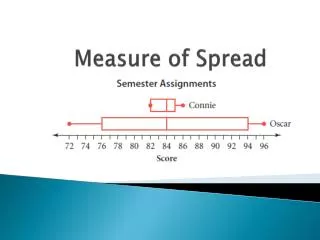
Measure of Spread . Lesson 2.2. Students Connie and Oscar from Exercises 7 and 8 in Lesson 2.1 had the same mean and median scores, but the ranges and IQR for their scores were very different. The range and IQR both measure the spread of the data.

E N D
Measure of Spread Lesson 2.2
Students Connie and Oscar from Exercises 7 and 8 in Lesson 2.1 had the same mean and median scores, but the ranges and IQR for their scores were very different. The range and IQR both measure the spread of the data.
The IQR describes the spread of data relative to the median. • It can also be useful to look at the spread relative to the mean. • One way to measure the spread of data relative to the mean is to calculate the deviations, the signed differences between the data values and the mean. • Recall the mean score for each student was 84.
What do the deviations tell you about each student’s performance?
A Good Design • In this investigation you will attempt to control the setup of an experiment in order to limit the variability of your results. • Select and perform one of these experiments. Make complete and careful notes about the setup of your experiment.
Experiment 1: Rolling Ball • In this experiment you’ll roll a ball of paper down a ramp and off the edge of your desk. • Build your ramp from books, notebooks, or a pad of paper. • Select the height and slope of your ramp and the distance from the edge of your desk, and determine any other factors that might affect your results. • Make a ball by crumpling a piece of paper, and roll it down the ramp. • Record the horizontal distance to the place where the ball hits the floor. • Repeat this procedure with the same ball, the same ramp setup, and the same release another seven or eight times.
Experiment 2: Rubber Band Launch • In this experiment you’ll use a ruler to launch a rubber band. • Select the height and angle of your launch and the length of your stretch, and determine any other factors that might affect your results. • Launch the rubber band into an area clear of obstructions. • Record the horizontal distance of the flight. • Repeat this procedure as precisely as you can with the same rubber band, the same launch setup, and the same stretch another seven or eight times.
Experiment 1 or 2 • Use your data from Experiment 1 or 2. Calculate the mean distance for your trials and then calculate the deviations. Mean (band)=169.2428 Mean (ball) =28.4
Deviation of the band = 16.951 Deviation of the ball = 6.943
Experiment 1 or 2 • In general, how much do your data values differ from the mean? • How does the variability in your results relate to how controlled your setup was? • Determine a way to calculate a single value that tells how accurate your group was at repeating the procedure. • Write a formula to calculate your statistic using the deviations. Deviation =average| sample – mean|
A value known as the standard deviation helps measure the spread of data away from the mean. Use your calculator to find this value for your data. Standard deviation for the band = 20.190332434349 Standard deviation for the ball = 8.8928810479694
What are the units of the statistic you calculated in Step 2? The units of the standard deviation you found in Step 3 are the same as those of the original measurements. How does your statistic compare to the standard deviation?
If you were going to repeat the experiment, how would you change your procedures to minimize the standard deviation?
Connie: {82, 86, 82, 84, 85, 84, 85} mean: 84 Oscar: {72, 94, 76, 96, 90, 76, 84} mean:84 Consider Connie’s and Oscar’s scores and their deviations from the mean score for each student. How can you combine the deviations into a single value that reflects the spread in a data set? Finding the sum is a natural choice. However, if you think of the mean as a balance point in a data set, then the directed distances above and below the mean should cancel out. Hence, the deviation sum for both Connie and Oscar is zero.
Connie: {82, 86, 82, 84, 85, 84, 85} mean: 84 Oscar: {72, 94, 76, 96, 90, 76, 84} mean:84 variance Standard deviation The standard deviation provides one way to judge the “average difference” between data values and the mean. It is a measure of how the data are spread around the mean.
In statistics, the mean is often referred to by the symbol . Another symbol, Σ , is used to indicate the sum of the data values. For example, Where are individual data. The mean of n data values is given by
Sigma notation is useful for defining standard deviation. The standard deviation, s, is a measure of the spread of a data set. where xi represents the individual data values, n is the number of values, and is the mean. The standard deviation has the same units as the data.
The larger standard deviation for Oscar indicates that his scores generally lie much farther from the mean than do Connie’s. A large value for the standard deviation tells you that the data values are not as tightly packed around the mean. As a general rule, a set with more data near the mean will have less spread and a smaller standard deviation.
You may wonder why you divide by (n -1) when calculating standard deviation. As you know, the sum of the deviations is zero. So, if you know all but one of the deviations, you can calculate the last deviation by making sure the sum will be zero. The last deviation depends on the rest, so the set of deviations contains only (n -1) independent pieces of data.
This table gives the student-to-teacher ratios for public elementary and secondary schools in the United States.
a. Calculate the mean and the standard deviation. What do the statistics tell you about the spread of the student-to-teacher ratios? Mean=15.546 SD = 2.48
More than half the ratios are within 2.48 students of the mean. Mean=15.55 Mean + SD =18.03 Mean - SD =13.07
Identify any values that are more than two standard deviations from the mean. What percentage of all values are more than two standard deviations from the mean?
There are no states that average fewer than 10.58 students per teacher. There are four states that exceed this value: OR (20.6), CA (21.1), AZ (21.3), and UT (22.4). So 4 out of 50 or 8%, of the states are more than two standard deviations from the mean. Mean=15.55 Mean + 2 SD = 20.51 Mean - 2 SD =10.58
Another Sample 1. The monthly averages of precipitation for Tucson, AZ, in inches, in a given year are 0.8, 0.8, 0.8, 0.2, 0.2, 0.4, 2.5, 2.7, 1.4, 1.1, 0.6, and1.1. a. Find the standard deviation.
1 out of 12 data are outside the 2 sd from the mean or 8.3% of the data Mean = 1.05 Mean +2SD= 2.6 Mean -2SD= -.5
Another Sample 1. The monthly averages of precipitation for Tucson, AZ, in inches, in a given year are 0.8, 0.8, 0.8, 0.2, 0.2, 0.4, 2.5, 2.7, 1.4, 1.1, 0.6, and1.1. a. Find the standard deviation. b. What percentage of the values are more than two standard deviations away from the mean? [8.3%]