Download
1 / 115
2.32k likes | 4.67k Vues
Chapter 2 FLUID STATICS. The science of fluid statics : the study of pressure and its variation throughout a fluid the study of pressure forces on finite surfaces Special cases of fluids moving as solids are included in the treatment of statics because of the similarity of forces involved.

E N D
The science of fluid statics : • the study of pressure and its variation throughout a fluid • the study of pressure forces on finite surfaces • Special cases of fluids moving as solids are included in the treatment of statics because of the similarity of forces involved. • Since there is no motion of a fluid layer relative to an adjacent layer, there are no shear stresses in the fluid • all free bodies in fluid statics have only normal pressure forces acting on their surfaces
2.1 PRESSURE AT A POINT • Average pressure: dividing the normal force pushing against a plane area by the area. • Pressure at a point: the limit of the ratio of normal force to area as the area approaches zero size at the point. • At a point: a fluid at rest has the same pressure in all directions an element δA of very small area, free to rotate about its center when submerged in a fluid at rest, will have a force of constant magnitude acting on either side of it, regardless of its orientation. • To demonstrate this, a small wedge-shaped free body of unit width is taken at the point (x, y) in a fluid at rest (Fig.2.1)
There can be no shear forces the only forces are the normal surface forces and gravity the equations of motion in the x and y directions px, py, ps are the average pressures on the three faces, γ is the unit gravity force of the fluid, ρ is its density, and ax, ay are the accelerations • When the limit is taken as the free body is reduced to zero size by allowing the inclined face to approach (x, y) while maintaining the same angle θ, and using the equations simplify to Last term of the second equation – infinitestimal of higher of smallness, may be neglected
When divided by δy and δx, respectively, the equations can be combined • θ is any arbitrary angle this equation proves that the pressure is the same in all directions at a point in a static fluid • Although the proof was carried out for a two-dimensional case, it may be demonstrated for the three-dimensional case with the equilibrium equations for a small tetrahedron of fluid with three faces in the coordinate planes and the fourth face inclined arbitrarily. • If the fluid is in motion (one layer moves relative lo an adjacent layer), shear stresses occur and the normal stresses are no longer the same in all directions at a point the pressure is defined as the average of any three mutually perpendicular normal compressive stresses at a point, • Fictitious fluid of zero viscosity (frictionless fluid): no shear stresses can occur at a point the pressure is the same in all directions
2.2 BASIC EQUATION OF FLUID STATICS Pressure Variation in a Static Fluid • Force balance: • The forces acting on an element of fluid at rest (Fig. 2.2): surface forces and body forces. • With gravity the only body force acting, and by taking the y axis vertically upward, it is -γδx δy δz in the y direction • With pressure p at its center (x, y, z) the approximate force exerted on the side normal to the y axis closest to the origin and the opposite e side are approximately δy/2 – the distance from center to a face normal to y
Figure 2.2 Rectangular parallelepiped element of fluid at rest
Summing the forces acting on the element in the y direction • For the x and z directions, since no body forces act, • The elemental force vector δF • If the element is reduced to zero size, alter dividing through by δx δy δz = δV, the expression becomes exact. • This is the resultant force per unit volume at a point, which must be equated to zero for a fluid at rest. • The gradient ∇ is
-∇p is the vector field f or the surface pressure force per unit volume • The fluid static law or variation of pressure is then • For an inviscid fluid in motion, or a fluid so moving that the shear stress is everywhere zero, Newton's second law takes the form a is the acceleration of the fluid element, f - jγ is the resultant fluid force when gravity is the only body force acting
In component form, Eq. (2.2.4) becomes The partials, for variation in horizontal directions, are one form of Pascal's law; they state that two points at the same elevation in the same continuous mass or fluid at rest have the same pressure. • Since p is a function of y only, relates the change of pressure to unit gravity force and change of elevation and holds for both compressible and incompressible fluids • For fluids that may be considered homogeneous and incompressible, γ is constant, and the above equation, when integrated, becomes in which c is the constant of integration. The hydrostatic law of variation of pressure is frequently written in the form h = -y, p is the increase in pressure from that at the free surface
Example 2.1 An oceanographer is to design a sea lab 5 m high to withstand submersion to 100 m, measured from sea level to the top of the sea lab. Find the pressure variation on a side of the container and the pressure on the top if the relative density of salt water is 1.020. At the top, h = 100 m, and If y is measured from the top of the sea lab downward, the pressure variation is #
Pressure Variation in a Compressible Fluid • When the fluid is a perfect gas at rest at constant temperature • When the value of γ in Eq. (2.2.7) is replaced by ρg and ρ is eliminated between Eqs. (2.2.7) and (2.2.9), • If P = P0 when ρ = ρ0, integration between limits - the equation for variation of pressure with elevation in an isothermal gas • - constant temperature gradient of atmosphere
Example 2.2 Assuming isothermal conditions to prevail in the atmosphere, compute the pressure and density at 2000 m elevation if P = 105Pa, ρ = 1.24 kg/m3 at sea level. From Eq. (2.2.12) Then, from Eq. (2.2.9) #
2.3 UNITS AND SCALES OF PRESSURE MEASUREMENT • Pressure may be expressed with reference to any arbitrary datum • absolute zero • local atmospheric pressure • Absolute pressure: difference between its value and a complete vacuum • Gage pressure: difference between its value and the local atmospheric pressure
The bourdon gage (Fig. 2.3): typical of the devices used for measuring gage pressures • pressure element is a hollow, curved, flat metallic tube closed at one end; the other end is connected to the pressure to be measured • when the internal pressure is increased, the tube tends to straighten, pulling on a linkage to which is attached a pointer and causing the pointer to move • the dial reads zero when the inside and outside of the tube are at the same pressure, regardless of its particular value • the gage measures pressure relative to the pressure of the medium surrounding the tube, which is the local atmosphere
Figure 2.4:the data and the relations of the common units of pressure measurement • Standard atmospheric pressure is the mean pressure at sea level, 760 mm Hg. • A pressure expressed in terms of the length of a column of liquid is equivalent to the force per unit area at the base of the column. The relation for variation of pressure with altitude in a liquid p = γh [Eq. (2.2.8)] (p is in pascals, γ in newtons per cubic metre, and h in metres) • With the unit gravity force of any liquid expressed as its relative density S times the unit gravity force of water: • Water: γ may be taken as 9806 N/m3.
Local atmospheric pressure is measured by • mercury barometer • aneroid barometer (measures the difference in pressure between the atmosphere and an evacuated box or tube in a manner analogous to the bourdon gage except that the tube is evacuated and sealed) • Mercury barometer: glass tube closed at one end, filled with mercury, and inverted so that the open end is submerged in mercury. • It has a scale: the height of column R can be determined • The space above the mercury contains mercury vapor. If the pressure of the mercury vapor hv is given in millimetres of mercury and R is measured in the same units, the pressure at A may be expressed as (mm Hg) Figure 2.5 Mercury barometer
Figure 2.4: a pressure may be located vertically on the chart, which indicates its relation to absolute zero and to local atmospheric pressure. • If the point is below the local-atmospheric-pressure line and is referred to gage datum, it is called negative, suction, or vacuum. • Example: the pressure 460 mm Hg abs, as at 1, with barometer reading 720 mm, may be expressed as -260 mm Hg, 260 mm Hg suction, or 260 mm Hg vacuum. • Note: Pabs = pbar + pgage • Absolute pressures : P, gage pressures : p.
Example 2.3 The rate of temperature change in the atmosphere with change in elevation is called its lapse rate. The motion of a parcel of air depends on the density of the parcel relative to the density of the surrounding (ambient) air. However, as the parcel ascends through the atmosphere, the air pressure decreases, the parcel expands, and its temperature decreases at a rate known as the dry adiabatic lapse rate. A firm wants lo burn a large quantity of refuse. It is estimated that the temperature of the smoke plume at 10 m above the ground will be 11oC greater than that of the ambient air. For the following conditions determine what will happen to the smoke. (a) At standard atmospheric lapse rate β = -0.00651oC per meter and t0 =20oC. (b) At an inverted lapse rate β = 0.00365oC per meter.
By combining Eqs. (2.2.7) and (2.2.14), The relation between pressure and temperature for a mass of gas expanding without heat transfer (isentropic relation, Sec. 6.1) is in which T1 is the initial smoke absolute temperature and P0 the initial absolute pressure; k is the specific heat ratio, 1.4 for air and other diatomic gases. Eliminating P/P0 in the last two equations Since the gas will rise until its temperature is equal to the ambient temperature, the last two equations may be solved for y. Let Then For β = -0.00651oC per metre, R = 287 m·N/(kg·K), a = 2.002, and y = 3201 m. For the atmospheric temperature inversion β = -0.00365oC per metre, a = -0.2721, and y = 809.2 m. #
2.4 MANOMETERS • Manometers are devices that employ liquid columns for determining differences in pressure. • Figure 2.6a: the most elementary manometer – piezometer • It measures the pressure in a liquid when it is above zero gage • Glass tube is mounted vertically so that it is connected to the space within the container • Liquid rises in the tube until equilibrium is reached • The pressure is then given by the vertical distance h from the meniscus (liquid surface) to the point where the pressure is to be measured, expressed in units of length of the liquid in the container. • Piezometer would not work for negative gage pressures, because air would flow into the container through the tube
Figure 2.6b: for small negative or positive gage pressures in a liquid • With this arrangement the meniscus may come to rest below A, as shown. Since the pressure at the meniscus is zero gage and since pressure decreases with elevation, units of length H2O • Figure 2.6c: for greater negative or positive gage pressures (a second liquid of greater relative density employed) • It must be immiscible in the first fluid, which may now be a gas • If the relative density of the fluid at A is S1 (based on water) and the relative density of the manometer liquid is S2, the equation for pressure at A hA - the unknown pressure, expressed in length units of water, h1, h2 - in length units
A general procedure in working all manometer problems : • Start at one end (or any meniscus if the circuit is continuous) and write the pressure there in an appropriate unit (say pascals) or in an appropriate symbol if it is unknown. • Add to this the change in pressure, in the same unit, from one meniscus to the next (plus if the next meniscus is lower, minus if higher). (For pascals this is the product of the difference in elevation in metres and the unit gravity force of the fluid in newtons per cubic metre.) • Continue until the other end of the gage (or the starting meniscus) is reached and equate the expression to the pressure at that point, known or unknown. • The expression will contain one unknown for a simple manometer or will give a difference in pressures for the differential manometer. In equation form,
A differential manometer (Fig. 2.7) determines the difference in pressures at two points A and B when the actual pressure at any point in the system cannot be determined • Application of the procedure outlined above to Fig. 2.7a produces • For Fig. 2.7b: • If the pressures at A and B are expressed in length of the water column, the above results can be written, for Fig. 2.7a, • For Fig 2.7b:
Example 2.4 In Fig. 2.7a the liquids at A and B are water and the manometer liquid is oil. S = 0.80; h1 = 300 mm; h2 = 200 mm; and h3 = 600 mm. (a) Determine pA - pB, in pacals. (b) If pB = 50kPa and the barometer reading is 730 mm Hg, find the pressure at A, in meters of water absolute. (a) (b) (a)
Micromanometers • For determining very small differences in pressure or determining large pressure differences precisely – several types of manometers • One type very accurately measures the differences in elevation of two menisci of a manometer. • By means of small telescopes with horizontal cross hairs mounted along the tubes on a rack which is raised and lowered by a pinion and slow motion screw so that the cross hairs can be set accurately, the difference in elevation of menisci (the gage difference) can be read with verniers.
Fig. 2.8: two gage liquids, immiscible in each other and in the fluid to be measured a large gage difference R can be produced for a small pressure difference. • The heavier gage liquid fills the lower U tube up to 0-0; then the lighter gage liquid is added to both sides, filling the larger reservoirs up to 1-1. • The gas or liquid in the system fills the space above 1-1. When the pressure at C is slightly greater than at D, the menisci move as indicated in Fig. 2.8. • The volume of liquid displaced in each reservoir equals the displacement in the U tube • Manometer equation γ1, γ2 and γ3 are the unit gravity force
Example 2.5 In the micromanometer of Fig 2.8 the pressure difference is wanted, in pascals, when air is in the system, S2 = 1.0, S3 = 1.10, a/A = 0.01, R = 5 mm, t = 20oC, and the barometer reads 760 mm Hg. The term γ1(a/A) may be neglected. Substituting into Eq. (2.4.1) gives #
Figure 2.9 Inclined manometer • The inclined manometer: frequently used for measuring small differences in gas pressures. • Adjusted to read zero, by moving the inclined scale, when A and B are open. Since the inclined tube requires a greater displacement of the meniscus for given pressure difference than a vertical tube, it affords greater accuracy in reading the scale. • Surface tension causes a capillary rise in small tubes. If a U tube is used with a meniscus in each leg, the surface-tension effects cancel.
2.5 FORCES ON PLANE AREAS • In the preceding sections variations oF pressure throughout a fluid have been considered. • The distributed forces resulting from the action of fluid on a finite area may be conveniently replaced by a resultant force, insofar as external reactions to the force system are concerned. • In this section the magnitude of resultant force and its line of action (pressure center) are determined by integration, by formula, and by use of the concept of the pressure prism.
Horizontal Surfaces • A plane surface in a horizontal position in a fluid at rest is subjected to a constant pressure. • The magnitude of the force acting on one side of the surface is • The elemental forces pdA acting on A are all parallel and in the same sense a scalar summation of all such elements yields the magnitude of the resultant force. Its direction is normal to the surface and toward the surface if p is positive. • Fig. 2.10: arbitrary xy axes - to find the line of action of the resultant, i.e., the point in the area where the moment of the distributed force about any axis through the point is zero, • Then, since the moment of the resultant must equal the moment of the distributed force system about any axis, say the y axis, x’ – the distance from the y axis to the resultant
Figure 2.10 Notation for determining the line of action of a force
Momentum (1) First moment • The moment of an area A about the y axis • The moment about a parallel axis, for example, x = k, the moment • Centroidal axis • Volume center • Mass center: center of gravity of a body
(2) Second moment • The moment about a parallel axis, for example, x = k, the moment • The second moment of an area A (the moment of inertia of the area) • Figure A.2 Moments of inertia of simple areas about centroidal axes
The product of inertia Ixy of an area - the product of inertia about centroidal axes parallel to the xy axes.
Inclined Surfaces • Fig. 2.11: a plane surface is indicated by its trace A'B‘;it is inclined θo from the horizontal. x axis: intersection of the plane of the area and the free surface. y axis: taken in the plane of the area, with origin O in the free surface. The xy plane portrays the arbitrary inclined area. The magnitude, direction, and line of action of the resultant force due to the liquid, acting on one side of the area, are sought. • For δA: • Since all such elemental forces are parallel, the integral over the area yields the magnitude of force F, acting on one side of the area, • Magnitude of force exerted on one side of a plane area submerged in a liquid is the product of the area and the pressure at its centroid • The presence of a free surface is unnecessary
Figure 2.11 Notation for force of liquid on one side of a plane inclined area.
Center of Pressure • Fig. 2.11: the line of action of the resultant force has its piercing point in the surface at a point called the pressure center, with coordinates (xp, yp). Center of pressure of an inclined surface is not at the centroid. To find the pressure center, the moments of the resultant xpF, ypF are equated to the moment of the distributed forces about the y axis and x axis, respectively - may be evaluated conveniently through graphical integration, for simple areas they may be transformed into general formulas:
When either of the centroidal axes is an axis of symmetry for the surface, vanishes and the pressure center lies on x=x- . Since may be either positive or negative, the pressure center may lie on either side of the line x = x-. To determine yp by formula, with Eqs. (2.5.2) and (2.5.6) • In the parallel-axis theorem for moments of inertia in which IG is the second moment or the area about its horizontal centroidal axis. If IG is eliminated from Eq. (2.5.9)
Example 2.6 The triangular gate CDE (Fig. 2.12) is hinged along CD and is opened by a normal force P applied at E. It holds oil, relative density 0.80, above it and is open to the atmosphere on its lower side Neglecting the weight of the gate, find (a) the magnitude of force exerted on the gate by integration and by Eq. (2.5.2); (b) the location of pressure center; (c) the force P needed to open the gate. Figure 2.12 Triangular gate
(a) By integration with reference to Fig. 2.12, When y = 4, x = 0, and when y = 6.5, x = 3, with x varying linearly with y; thus in which the coordinates have been substituted to find x in terms of y. Solving for a and b gives Similarly, y = 6.5, x = 3; y = 9, x = 0; and x = 6/5(9 - y). Hence, Integrating and substituting for γsinθ leads to By Eq. (2.5.2)
(b) With the axes as shown, In Eq. (2.5.8) I-xyis zero owing to symmetry about the centroidal axis parallel to the x axis; hence In Eq. (2.5.11), i.e., the pressure center is 0.16 m below the centroid, measured in the plane of the area. (c) When moments about CD are taken and the action of the oil is replaced by the resultant,
The Pressure Prism • Pressure prism: another approach to determine the resultant force and line of action of the force on a plane surface - prismatic volume with its base the given surface area and with altitude at any point of the base given by p = γh. h is the vertical distance to the free surface, Fig. 2.13. (An imaginary free surface may be used to define h if no real free surface exists.) (in the figure, γh may be laid off to any convenient scale such that its trace is OM) • The force acting on an elemental area δA is (2.5.12) - an element of volume of the pressure prism. After integrating, F = ϑ • From Eqs. (2.5.5) and (2.5.6), (2.5.13) xp, yp are distances to the centroid of the pressure prism the line of action of the resultant passes through the centroid of the pressure prism