Chapter 5. The Amorphous State
Chapter 5. The Amorphous State. 5.1 The Amorphous Polymer State. Bulk state condensed state, solid state Includes both amorphous and crystalline polymers. 5.1.1 Solids and Liquids.

Chapter 5. The Amorphous State
E N D
Presentation Transcript
5.1 The Amorphous Polymer State Bulk state condensed state, solid state Includes both amorphous and crystalline polymers. 5.1.1 Solids and Liquids An amorphous polymer does not exhibit a crystalline X-ray diffraction pattern, and it does not have a first-order melting transition. 5.1.2 Possible Residual Order in Amorphous Polymers?
5.2 Experimental Evidence Regarding Amorphous Polymers Short-range interactions ~ 2 nm Long-range interactions 5.2.1 Short-Range Interactions in amorphous Polymers • Method that measure short-range interactions can be divided into two groups: • those measure the orientation or correlation of the mers along the axialdirection of a chain, • (ii) those that measure the order between chains, in the radialdirection.
There are several measures of the axial direction : Kuhn segment length Persistence length as the length down a chain from a given point where the polymer’s direction is random with respect to starting point. The value of the persistence length for polyethylene is 0.575 nm.
One of the most powerful experimental methods of determining short-range order in polymers utilizes birefringence. The birefringence of a sample is defined by Where n1 and n2 are the refractive indexes for light polarized in two directions 90o apart. If polymer sample is stretched, n1and n2 are taken as the refractive indexes for light polarized parallel and perpendicular to the stretching direction.
The anisotropy of refractive index of the stretched polymer can be demonstrated by placing a thin film between crossed polaroids. For stretching at 45oto the polarization directions, the fraction of light transmitted is given by d represents the thickness and lo represents the wavelength of light in vacuum.
By measuring the transmitted light quantitatively, the birefringence is obtained. The birefringence is related to the orientation of molecular units such as mers, crystals, or even chemical bonds by Where fi is an orientation function of such units given by Whereqi is the angle that the symmetry axis of the unit makes with respect to the stretching direction. b1 and b2 are the polarizabilities along and perpendicular to the axes of such units.
Equation (5.4) contains two important solutions for fibers and films: The stress-optical coefficient (SOC) is a measure of the change in birefringence on stretching sample under a stress s If the polymer is assumed to obey rubbery elasticity relations, then
5.2.2 Long-Range Interactions in amorphous Polymers 5.2.2.1 Small-Angle Neutron Scattering Applied to polymers, SANS techniques can be used to determine the actual chain radius of gyration in the bulk state. P(Q) : form factor
In SAS experiments, a deuterated polymer is dissolved in an ordinary hydrogen-bearing polymer of the same type. As currently used, the coherent intensity in a SANS experiment is described by the cross section, dΣ/dΩ, which is the probability that a neutron will be scattered in a solid angle, Ω, per unit volume of the sample. Where CN, the analogue of H, may be expressed
Zero effective interaction: ‘ideal’ chain 1.4. Fractal (self-similar) nature of polymer conformation Attraction: collapsed chain Short-range repulsion: expanded chain Long-range repulsion: extended chain
Hard sphere/full 3D body: m ~ r3 Hard disk/full 2D sheet: m ~ r2 Rigid rod/full straight line: m ~ r Fractal structure: m ~ rD
4A•(r2)D = 4•m2 = m1 = A•r1D = A•(3r2)D • (3r2)D = 4•(r2)D 3D = 4 D = ln4/ln3 = 1.26
3A•(r2)D = 3•m2 = m1 = A•r1D = A•(2r2)D • (2r2)D = 3•(r2)D • (2)D = 3 D = ln3/ln2 = 1.58
g ~ <r2> ~ (<r2>1/2)D D = 2
Within a proper length (or q) range, I ~ qD (mass fractals, D = 1 to 3) I ~ q6-D (surface fractals, D = 3-4) Mass fractal dimension D = ca. 2 Surface fractal dimension D = ca. 2
Slope = ca. 1.8 Mass fractal dimention D = 1.8
g ~ (<r2>1/2)D <r2>1/2 ~ g1/D 1/D 0.5 0.75 0.588 0.25 0.625 0.5 0.527 0.4
5.2.2.2 Electron and X-Ray Diffraction The diffraction in amorphous is much more diffuse, sometimes called halos.
Polytetrafluoroethylene was found to have more or less straight chains in the axial direction for distances of at least 2.4 nm.
The greater interchain spacing of polystyrene and silicone rubbers is in part caused by bulky side groups compared with polyethylene.
5.2.2.3 General Properties Two of the most important general properties of the amorphous polymers are the density and the excess free energy due to non-attainment of equilibrium. For many common polymers the density of the amorphous phase is approximately 0.85 to 0.95 that of the crystalline phase.
5.3 Conformation of the Polymer Chain 5.3.1 Models and Ideas 5.3.1.1 The Freely Jointed Chain The simplest mathematical model of a polymer chain in space is the freely jointed chain. It has n links, each of length l, jointed in a linear sequence with no restrictions on the angles between successive bonds. By analogy with Brownian motion statistics, the root-mean –square end-to-end distance is given by
A more general equation yielding the average end-to-end distance of a random coil, ro, is given by Where Θ is the bond angle between atoms, and φ is the conformational angle. Long-range interactions include excluded volume, which eliminates conformations in which two widely separated segments would occupy the same space. The total expansion is represented by a constant, C∞, after squaring both sides of equation (5.12):
The characteristic ratio C∞ = r2/l2n varies from about 5 ~ 10, depending on the foliage present on the individual chains
5.3.1.2 Kuhn Segments There are several approaches for dividing the polymer chain into specified lengths for conceptual or analytic purposes. The Kuhn segment length, b, depends on the chain’s end-to-end distance under Flory Q-conditions, or its equivalent in the unoriented, amorphous bulk state, rQ, Where L represents the chain contour length For flexible polymers, the Kuhn segment size varies between 6 and 12 mers, having a value of 8 mers for PS, and 6 for PMMA. The Kuhn segment also expresses the idea of how far one must travel along a chain until all memory of starting direction is lost.
5.3.2 The Random Coil The term “random coil” is often used to describe the unperturbed shape of the polymer chains in both dilute solution and in the bulk amorphous state. In dilute solutions the random coil dimensions are present under Flory Q-solvent conditions, where the polymer-solvent interactions and excluded volume terms just cancel each other. In the bulk amorphous state the mers are surrounded entirely by identical mers, and the sum of all the interactions is zero. In the limit of high molecular weight, the end-to-end distance of a random coil divided by the square root of 6 yield the Rg.
5.4 Macromolecular Dynamics Polymer motion can take two forms: (a) the chain can change its overall conformation, as in relaxation after strain, or (b) it can move relative to its neighbors. Polymer chains find it almost impossible to move “sideways” by simple translation, for such motion is exceedingly slow for long, entangled chains.
The first molecular theories concerned with polymer chain motion were developed by Rouse and Bueche. Polymer chain may be considered as a succession of equal submolecules, each long enough to obey the Gaussian distribution function. The Rouse-bueche theory is useful especially below 1%concentration. However, only poor agreement is obtained on studies of bulk melt.
5.4.1 The Rouse-Bueche Theory These submolecules are replaced by a series of beads of mass M connected by springs with the proper Hook’s force constant. In the development of rubber elasticity theory, it will be shown that the restoring force, f, on a chain or chain portion large enough to be Gaussian, is given by Where Δx is the displacement and r is the end-to-end distance of the chain.
If the beads are numbered 1,2,3…,z, so that there are z springs and z+1 beads, the restoring force on the ith bead may be written The segments move through a viscous medium, this viscous medium exerts a drag force on the system, damping out the motions. The viscous force on the ith bead is given by Where r is the friction factor Relaxation time is
5.4.2 Reptation and Chain Motion 5.4.2.1 The de Gennes Reptation Theory This model consisted of a single polymeric chain, P, trapped inside a three-dimensional network, G, such as a polymer gel.
The snakelike motion is called reptation. The chain is assumed to have certain “defects”, each with stored length, b. These defects migrate along the chain in a type of defect current. The velocity of the nth mer is related to the defect current Jn by Where rn represents the position vector of the nth mer Using scaling concepts, the self-diffusion coefficient, D, of a chain in the gel depends on the molecular weight M as
The reptation time, Tr, depends on the molecular weight as Doi and Edwards developed the relationship of the dynamics of reptating chains to mechanical properties. shear modulus steady state viscosity compliance
5.4.2.2 Fickian and Non-Fickian Diffusion The three-dimensional self-diffusion coefficient, D, of a polymer chain in a melt is given by Where X is the center-of-mass distance traversed in three dimensions, and t represents the time.
5.4.3 Nonlinear Chains How do branched, star, and cyclic polymers diffuse? Two possibilities exist for translational motion in branched polymers. First, one end may move forward, pulling the other end the the branch into the same tube. It is energetically cheaper for an entangled branched-chain polymer to renew its conformation by retracting a branch so that it retraces its path along the confining tube to the position of the center mer.