Estimating Surface Normals in Noisy Point Cloud Data
Estimating Surface Normals in Noisy Point Cloud Data. Niloy J. Mitra, An Nguyen. Stanford University. The Normal Estimation Problem. Given Noisy PCD sampled from a curve/surface. The Normal Estimation Problem. Given Noisy PCD sampled from a curve/surface

Estimating Surface Normals in Noisy Point Cloud Data
E N D
Presentation Transcript
Estimating Surface Normals in Noisy Point Cloud Data Niloy J. Mitra, An Nguyen Stanford University
The Normal Estimation Problem • GivenNoisy PCD sampled from a curve/surface
The Normal Estimation Problem • GivenNoisy PCD sampled from a curve/surface • GoalCompute surface normals at each point p Error bound the normal estimates
A Standard Solution Use least square fit to a neighborhood of radius r around point p
A Standard Solution Use least square fit to a neighborhood of radius r around point p PROBLEM !!what neighborhood size to choose?
Contributions of this paper • Study the effects of curvature, noise, sampling density on the choice of neighborhood size. • Use this insight to choose an optimal neighborhood size. • Compute bound on the estimation error.
Outline • Problem statement • Related work • Neighborhood Size Estimation • Analysis in 2D and 3D • Applications • Future Work
Related Work • Surface reconstruction • crust, cocone, etc • Guarantees about the surface normals • Mostly works in absence of noise • Curve/Surface fitting • pointShop3D, point-set • Works in presence of noise • Performance guarantees?
aTp=c Least Square Fit • Assume best fit hyperplane: aTp=c • Minimize • Reduces to the eigen-analysis ofthe covariance matrix • Smallest eigenvector of M is the estimate of the normal
Collusive noise Deceptive Case
Collusive noise Curvature effect Deceptive Cases
Outline • Problem statement • Related work • Neighborhood Size Estimation • Analysis in 2D and 3D • Applications • Future Work
Assumptions • Noise • Independent of measurement • Zero mean • Variance is known (noise need not be bounded) • Data • Sampling criterion satisfied • Evenly distributed data • To prevent biased estimates • Curvature is bounded
Sampling Criteria (2D) • Sampling density • lower bound (like Nyquist rate) • upper bound (to prevent biased fits) Evenly distributed Number of points in a disc of radius r bounded above and below by (1)r (,) sampling condition [Dey et. al.] implies evenly distributed.
O y x 2r Modeling (2D) • At a point O • Points of PCD inside a disc of radius r comes from a segment of the curve • y = g(x) define the curve for all x[-r,r] • Bounded curvature: |g’’(x)|< for all x • Additive Noise(n) in y-direction (x,g(x)+n) • r, n/r assumed to be small
Proof Idea • Eigen-analysis of covariance matrix
Proof Idea • covariance matrix • let, =(|m12|+m22)/m11
Proof Idea • covariance matrix • let, =(|m12|+m22)/m11 • error angle bounded by, • to bound estimation error, need to bound
Bounding Terms of M • For evenly distributed samples it follows,
Bounding m12 • Evenly sampled distribution • Noise and measurement are uncorrelated • E(xn)= E(x)E(n)= 0 • Var(xn)= (1)r2n2 • Chebyshev Inequality • bound with probability (1-) • Finally,
Bounding Estimation Error =(|m12|+m22)/m11
Final Result in 2D • = 0, • take as large a neighborhood as possible
Final Result in 2D • = 0, take as large a neighborhood as possible • n= 0 • take as small a neighborhood as possible
Result for 3D A similar but involved analysis results in, A good choice of r is,
How can we use this result? • Need to • know • estimate suitable values for • estimate locally
Estimating c1, c2 Exact normals known at almost all points • c1=1, c2=4 • same constants used for • following results
Algorithm • For each point, start with k =15 • Iterate and refine (maximum of 10 steps) • Compute r, , [Gumhold et al.] locally • Use them to compute rnew • knew = rnew2 old • Stop if • k>threshold • ksaturates
Effect of Noise on Neighborhood Size 2x noise 1x noise
Estimation Error > 5 o 2x noise 1x noise
Increasing Noise Can still get good estimates in flat areas 1x noise 2x noise 4x noise
Future Work • How to find a suitable neighborhood size for good curvature estimation • Find a better way for estimating c1, c2 • Design of a sparse query data structure for quick extraction of normal, curvature, etc from PCDs
Different Noise Distribution (same variance) gaussian uniform
Result: phone 1x noise
Varying neighborhood size Neighborhood size at all points being shown using color-coding. Purple denotes the smallest neighborhood and turns blue as the neighborhood size increases