Nonlinear Relationships
Nonlinear Relationships. Nonlinear relationships can be modeled by including a variable that is a nonlinear function of an independent variable. For example it is usually assumed that health care expenditures increase at an increasing rate as people age. Nonlinear Relationships.

Nonlinear Relationships
E N D
Presentation Transcript
Nonlinear Relationships Nonlinear relationships can be modeled by including a variable that is a nonlinear function of an independent variable. For example it is usually assumed that health care expenditures increase at an increasing rate as people age.
Nonlinear Relationships In that case you might try including age squared into the model: Health expend = 500 + (5)Age + (.5)AgeSQ Age Health Expend 600 20 800 30 1100 40 1500
Nonlinear Relationships If the dependent variable increases at a decreasing rate as the independent variable rises you might want to include the square root of the independent variable. If you are unsure of the nature of the relationship you can use dummy variables for different ranges of values of the independent variable.
Non-continuous Relationships If the relationship between the dependent variable and an independent variable is non-continuous a slope dummy variable can be used to estimate two sets of coefficients and intercepts for the independent variable. For example, if natural gas usage is not affected by temperature when the temperature rises above 60 degrees, we could have: Gas usage = b0 + b1(GT60) + b2(Temp) + b3(GT60)(Temp)
Non-continuous Relationships Note that at temperatures above 60 degrees the net effect of a 1 degree increase in temperature on gas usage is -0.056 (-.866+.810)
Interaction Terms You can try to control for interactions between two variables by including a variable that is the product of two independent variables. For example, assume we were estimating the salaries of baseball players. If there was a premium paid to players that were both good fielders and good hitters, we might want to include an interaction term for hitting and fielding in the model.
Standardized Coefficients Unstandardized Standardized Coefficients Coefficients B Std. Error Beta t Sig. (Constant) -14.485 4.038 -3.587 .000 Weight -.007 .000 -.706 -14.177 .000 Year .761 .050 .360 15.262 .000 Cylinders -.074 .232 -.016 -.320 .749 a Dependent Variable: MPG When the regression model is estimated after standardizing the values of the dependent and independent variables. Used to compare the magnitude of the effects of the independent variables.
Standardized Residuals Where s is the standard error of estimate and hi is the leverage of observation i. Leverage is determined by the difference between the value of the independent variables and their means.
Standardized Residuals The random deviation in the value of y, e, is assumed to be normally distributed. Looking at the standardized residuals gives some indication if that is true. Values should lie within 2 standard deviations of 0. Values greater than 2 may indicate the presence of outliers.