HIPPO: CO 2 and O 2 Analysis Plans
410 likes | 605 Vues
HIPPO: CO 2 and O 2 Analysis Plans. Britton Stephens (NCAR EOL) and HIPPO Science Team. Climate projections are sensitive to human decisions, and physical and carbon cycle feedbacks. Uncertainty due to climate models. }. Uncertainty due to trees and oceans. [IPCC, 2007].

HIPPO: CO 2 and O 2 Analysis Plans
E N D
Presentation Transcript
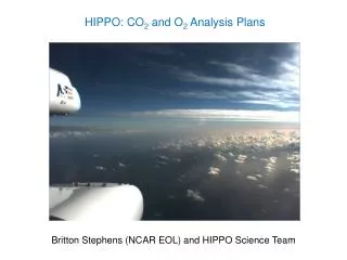
HIPPO: CO2 and O2 Analysis Plans Britton Stephens (NCAR EOL) and HIPPO Science Team
Climate projections are sensitive to human decisions, and physical and carbon cycle feedbacks Uncertainty due to climate models } Uncertainty due to trees and oceans [IPCC, 2007] Uncertainty due to people
Tropical Land and Northern Land fluxes plotted versus annual-mean northern-hemisphere vertical CO2 gradient Continental-scale carbon fluxes inferred from surface data are still very uncertain, owing to biases in atmospheric CO2 transport [Gurney et al., 2004; Stephens et al., 2007]
PIs: Harvard, NCAR, Scripps, NOAA • Global and seasonal survey of CO2, O2, CH4, CO, N2O, H2, SF6, COS, CFCs, HCFCs, O3, H2O, CO2 isotopes, Ar, black carbon, and hydrocarbons • NSF / NCAR Gulfstream V • 5 campaigns over 4 years • Continuous profiling from surface to 10 km and to 15 km twice per flight • hippo.ucar.edu (also Facebook, Twitter, YouTube) 67 S, Southern Ocean Pago Pago, American Samoa Brooks Range, Alaska
A global mission has 11 flight segments in 3 weeks; denotes PBL sample (~ 150 in each global program). HIPPO_2 Nov 2009 preHIPPO Apr-Jun 2008 HIPPO_3 Mar-Apr 2010 HIPPO_1 Jan 2009
Harvard/Aerodyne - QCLS CO2, CH4, CO, N2O (1 Hz) NCAR AO2 O2:N2 , CO2 (1 Hz) Harvard OMS CO2 CO2 (1 Hz) NOAA CSD O3 O3 (1 Hz) NOAA GMD O3 O3 (1 Hz) NCAR RAF CO CO (1 Hz) NOAA- UCATS, PANTHER GCs (1 per 70 – 200 s) CO, CH4, N2O, CFCs, HCFCs, SF6, CH3Br, CH3Cl, H2, H2O Whole air sampling: NWAS (NOAA), AWAS (Miami), MEDUSA (NCAR/Scripps) O2:N2, CO2, CH4, CO, N2O , other GHGs, CO2 isotopes, Ar/N2, COS, halocarbons, solvent gases, marine emission species, many more Princeton/SWS VCSEL H2O (1 Hz) NOAA SP2 Black Carbon (1 Hz) MTP, wing stores, etc T, P, winds, aerosols, cloud water HIPPO Aircraft Instrumentation – over 100 measurements of over 80 unique species
Oct-Jan Mar-Jun Jul-Sep
Without improving transport models, or waiting for them to be improved, there are already metrics that can be applied independent of transport errors: • Interannual variability • Terrestrial CO2: Growing season net flux (GSNF) and dormant season net flux (DSNF) • Oceanic O2: Seasonal net outgassing (SNO), seasonal net ingassing (SNI) • Tracer-tracer correlations (e.g. O2:CO2 ratios)
LEF LEF Column Average [Gurney et al., GBC 2004] “vertically-integrated observations . . . provide a measure of CO2 variations that is not highly sensitive to error in the transport fields. As a group, the seasonal cycle in column CO2 is most sensitive to the seasonal fluxes themselves.” TCCON data now calibrated using HIPPO “(unoptimized) CASA underestimates GSNF by ~ 25%” [Yang et al., GRL 2007]
Using light-aircraft profile data: “Surface-optimized CASA underestimates GSNF by 15%” [Nakatsuka and Maksyutov, BGS 2009] Have successfully said what the world is not (CASA), now let’s say what it is – define hemispheric GSNF and DSNF over multiple years “Our simulations suggest that boreal growing season NEE (between 45-65°N) is underestimated by ~40% in CASA.” TCCON data now calibrated using HIPPO [Keppel-Aleks, et al., Biogeosci., 2011]
Hypothesis: like column averages, integrated HIPPO slices are also much less sensitive to atmospheric transport errors. • Plan: • Average HIPPO CO2 over Northern Hemisphere for 9 slices • Model runs to test hypothesis • Combined analysis with TCCON and light-aircraft profile data • Goal: • GSNF and DSNF values as a rigid constraint on global ecosystem models
Without improving transport models, or waiting for them to be improved, there are already metrics that can be applied independent of transport errors: • Interannual variability • Terrestrial CO2: Growing season net flux (GSNF) and dormant season net flux (DSNF) • Oceanic O2: Seasonal net outgassing (SNO), seasonal net ingassing (SNI) • Tracer-tracer correlations (e.g. O2:CO2 ratios)
Seasonal Net Outgassing [Keeling and Shertz, Nature 1992] [Najjar and Keeling, GBC 2000] [Garcia and Keeling, JGR 2001]
Atmospheric Potential Oxygen (O2 + 1.1 * CO2) highlights oceanic exchange processes per meg ↑ Dissolved O2 climatology performed well in comparison to surface stations but appears to overestimate outgassing when airborne data included ORCA-PISCES-T underestimates → outgassing in December, but overestimates seasonal fluxes (as seen in H2 and H3), suggesting timing issues
10 Transcom models forced with a common seasonal ocean O2 flux field differ on surface concentration amplitude by a factor of 2. T. Blaine Dissertation, 2005
J. Bent, dissertation in progress Altitude-latitude integrated 180 W slices are equivalent to zonal means Models converge on predictions of seasonal amplitudes for altitude-latitude integrated 180 W slices
Conclusions • HIPPO data provide critical tests of global atmospheric transport models as well as constraints on surface fluxes that are independent of atmospheric transport model differences. • For CO2, winter build-up pervades the entire NH troposphere, with efficient mixing from low latitude/altitude to high latitude/altitude, whereas models tend to trap high CO2 near the surface in winter. • The NCAR AO2 instrument has detected the broad influence of Southern Ocean O2 fluxes for the first time, providing important constraints on ocean biogeochemistry and tests for models of carbon/climate feedbacks. • Other science highlights to date have included Arctic CH4 fluxes, tropical N2O fluxes, global H2O transport, and black carbon distributions. • With over 80 other species measured, many additional research avenues can be followed.
HIPPO Science Team: Harvard University: S. C. Wofsy, B. C. Daube, R. Jimenez, E. Kort, J. V. Pittman, S. Park, R. Commane, Bin Xiang, G. Santoni; (GEOS-CHEM) D. Jacob, J. Fisher, C. Pickett-Heaps, H. Wang, K. Wecht, Q.-Q. Wang National Center for Atmospheric Research: B. B. Stephens, S. Shertz, P. Romashkin, T. Campos, J. Haggerty, W. A. Cooper, D. Rogers, S. Beaton , R. Lueb NOAA ESRL and CIRES: J. W. Elkins, D. Fahey, R. Gao, F. Moore, S. A. Montzka, J. P. Schwartz, D. Hurst, B. Miller, C. Sweeney, S. Oltmans, D. Nance, E. Hintsa, G. Dutton, L. A. Watts, R. Spackman, K. Rosenlof, E. Ray UCSD/Scripps: R. Keeling, J. Bent Princeton: M. Zondlo, Minghui Diao U. Miami: E. A. Atlas TCCON: Vanessa Sherlock et al. JPL: M. J. Mahoney; (AIRS) M. Chahine, E. Olsen Cooperating modeling groups: ACTM P. Patra, K. Ishijima; GEMS-MACC R. Engelen; TM3/TM5 Sara Mikaloff-Fletcher;
Carbon Cycle Highlight: CH4 release from Arctic ecosystems There is very strong interest in determining if Arctic warming is leading to large releases of CO2 and CH4. But strong pollution inputs into the Arctic mask these diffuse emissions. The HIPPO-2 transect in early November was a golden time to study this phenomenon: soils were still warm, but biomass fires were over and the Arctic airmass did not yet cover northern pollution sources. We found very strong pollution signals high in the Arctic atmosphere (blue points, a surprise in itself), and the unmistakable signature of non-pollution inputs in the lower atmosphere over the whole Arctic Basin (red points). (E. Kort, S. Wofsy, Harvard)
500m 4500m N2O 321 323 325 -80 -60 -20 0 20 40 60 80 Highlights: Sources of N2O The observed distribution of N2O was completely different than predicted by models, even those that gave excellent results when inverted using surface data, and which did well for SF6. Inverse modeling using the ACTM model of P. Patra and K. Ishijima showed that N2O from strong sources in S. and S. E. Asia are lofted into the middle tropical troposphere. Since this part of the distribution had never been seen before, models did not previously attribute global sources correctly. (E. Kort, Harvard; P. Patra, K. Ishijima (JAMSTEC))
Highlights: Black CarbonApril 2010 HIPPO-3, April 2010 Southbound • Asian pollution lofted high into the Arctic troposphere; "blackened" atmosphere in November, 2009. • Biomass burning plumes from SE Asia contributed to gigantic BC loadings between ITCZ and ~40°N RAQMS CO simulation Biomass-burning from SE Asia • Very low BC loadings in southern hemisphere (SH)—much lower than models • Large BC loadings in northern hemisphere (NH) with loadings comparable to those in urban areas, originating in SE Asia (movie) • Strong interhemispheric gradient at the ITCZ Low BC in SH BC results from J Schwarz, R. Spackman, D. Fahey (NOAA); Movie courtesy Brad Pierce, NOAA
Carbon Cycle Highlight: CH4 release from Arctic ecosystems There is very strong interest in determining if Arctic warming is leading to large releases of CO2 and CH4. But strong pollution inputs into the Arctic mask these diffuse emissions. The HIPPO-2 transect in early November was a golden time to study this phenomenon: soils were still warm, but biomass fires were over and the Arctic airmass did not yet cover northern pollution sources. We found very strong pollution signals high in the Arctic atmosphere (blue points, a surprise in itself), and the unmistakable signature of non-pollution inputs in the lower atmosphere over the whole Arctic Basin (red points). (E. Kort, S. Wofsy, Harvard)
color scales differ Carbon Cycle Highlight: CO2 Seasonal cycle propagation Inverse models of the carbon cycle give conflicting results in part because they rely on data from surface stations, and various models give different results for the rate of propagation of seasonal changes in the middle troposphere. Data from November and January show the Arctic filling up with CO2 rapidly, with seasonal signals transported isentropically, rather than vertically or horizontally (note the vertical axis is Potential Temperature). Accurate representation of the "warm conveyor belt", and other jet-stream phenomena, may hold the key to improved CO2 modeling. (B. Stephens, NCAR)
500m 4500m 500m 4500m N2O 321 323 325 SF6 6.4 6.6 6.8 -80 -60 -20 0 20 40 60 80 Latitude -80 -60 -20 0 20 40 60 80 Highlights: Sources of N2O The observed distribution of N2O was completely different than predicted by models, even those that gave excellent results when inverted using surface data, and which did well for SF6. Inverse modeling using the ACTM model of P. Patra and K. Ishijima showed that N2O from strong sources in S. and S. E. Asia are lofted into the middle tropical troposphere. Since this part of the distribution had never been seen before, models did not previously attribute global sources correctly. (E. Kort, Harvard; P. Patra, K. Ishijima (JAMSTEC))
Highlights: Black CarbonApril 2010 HIPPO-3, April 2010 Southbound • Asian pollution lofted high into the Arctic troposphere; "blackened" atmosphere in November, 2009. • Biomass burning plumes from SE Asia contributed to gigantic BC loadings between ITCZ and ~40°N RAQMS CO simulation Biomass-burning from SE Asia • Very low BC loadings in southern hemisphere (SH)—much lower than models • Large BC loadings in northern hemisphere (NH) with loadings comparable to those in urban areas, originating in SE Asia (movie) • Strong interhemispheric gradient at the ITCZ Low BC in SH BC results from J Schwarz, R. Spackman, D. Fahey (NOAA); Movie courtesy Brad Pierce, NOAA
HIPPO O2 Highlight: Atmospheric Potential Oxygen (O2 + 1.1 * CO2) highlights oceanic exchange processes per meg ↑ Dissolved O2 climatology performed well in comparison to surface stations but appears to overestimate outgassing when airborne data included ORCA-PISCES-T underestimates → outgassing in December, but overestimates seasonal fluxes (as seen in H2 and H3), suggesting timing issues
Notable features of the mission • Very strong interest from modeling groups, rapid sharing of observations and model results. • Few operational issues (so far…). • Tall poles identified, solved, in advance. • Strong NCAR EOL/RAF management, Mission Manager (PavelRomashkin), flight crew; adaptation to unusual mission profile. • Success of HAIS sensors. • Strong science team. • Outreach via social media, professional website.
Data management Pre-release data • Merged data sets to the team within 24 hours. • Provisional data to cooperating modeling groups (i.e. anyone asking) and TCCON within 6-8 weeks. Data Release • Data management at NCAR (Janine Aquino) • Public portal, metadata, data protocol at CDIAC (Tom Boden, Sig Christensen) • Outreach website, social media (Allison Rockwell)
Websites for HIPPO • HIPPO Project Page (http://www.eol.ucar.edu/hippo/ ) full data sets, links to all of the sites • Outreach (http://hippo.ucar.edu ) • Public Portal at CDIAC (http://hippo.ornl.gov/ ) • Instant turnaround via postings on http://www.seas.harvard.edu/~swofsy and http://www.eol.ucar.edu/raf/Stephens/VTCO2 • Moving-target data upload and download (team use): ftp to/from : catalog.eol.ucar.edu
Species measured by PANTHER and UCATS Fred Moore, Eric Hintsa, Dale Hurst, Jim Elkins PANTHER (6-Channel GC): ECD channels: N2O, SF6, CCl2F2 (CFC-12),) CCl3F (CFC-11), and CBrClF2 (halon-1211) injected every 70 seconds, and H2, CH4, CO, CCl4, CH3CCl3 (methyl chloroform) and PAN (peroxyl acetyl nitrate) injected every 140 seconds. The width of a sample load on an ECD channel is only 3 seconds, allowing this data set to correlate well with other fast measurements. MSD channels: The methyl halides CH3I, CH3Br, CH3Cl, the sulfur compounds COS, CS2, the hydrochlorofluorocarbons CHClF2 (HCFC-22), C2H3Cl2F (HCFC-141b), C2H3ClF2 (HCFC-142b), and the hydrofluorocarbon C2H2F4 (HFC-134a) are injected every 180 seconds with 150 seconds sample load width. This data set correlates with a time average of other fast measurements. UCATS: 2-Channel GC: every 70 s (N2O, SF6) or every 140 s (H2, CH4, CO) TDL: 10-second average H2O Photometer: 1-Hz O3
Complete List of Chemical Species Monitored by the Whole Air Sampler (WAS) Elliot Atlas, Ben Miller, Steve Montzka