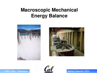
Macroscopic Mechanical Energy Balance Equations
150 likes | 228 Vues
Learn the principles of macroscopic energy balance, including accumulation, In-Out+Generation-Consumption, how energy enters a system, various forms of energy transfers, mechanisms of energy flow, and the historical context of Bernoulli's equation.

Macroscopic Mechanical Energy Balance Equations
E N D
Presentation Transcript
Macroscopic Energy Balance Accumulation = In – Out + {Generation – Consumption} Assume: • Energy is conserved • Steady State
Macroscopic Energy Balance How may Energy enter System? • Via Mass Flow • KE • PE • Int. Energy • Heat Transfer (Q) • Conduction • Radiation • Work on or by System (W) • Pumps • Compressors Note: Q and W positive for energy into system •
Energy Transferred via Mass Flow Convective Term • Internal Energy • Kinetic Energy • Potential Energy Flow Work Term • Pressure work requiredto push fluid through system
Variable Velocity at Cross Section Again integrate across cross section and introduce correction factor, a, to allow use of average velocity.
Variable Velocity at Cross Section Laminar FlowParabolic Flow α= 2 Turbulent FlowPlug Flow α≈
MEB with Correctionfor Variable Velocity Historical Note: Though this result is often called the Bernoulli equation, Bernoulli actually only considered W = hf = 0. ˆ Daniel Bernoulli (1700 - 1782)
Example 1 Determine the sign of the individual contributions to the MEB for the following:
Example 2 - Bernoulli and the airplane Cessna 172
Cessna 172 Data • Gross weight = 2300 lbs • Normal cruising speed = 65 mph • Wing surface area = 160 ft2 • Upper wing path length = 1.016 X lower wing path length
Mechanical Energy Balance 10 minute problem Water with a density of 998 kg/m3 is flowing at a steady mass rate through a uniform diameter pipe. The Reynolds number in the pipe is approximately 4000. The pump supplies 155.4 J/kg of fluid flowing through the pipe. Given the other conditions shown on the diagram, calculate the viscous dissipation, hf, in the pipe system.