Download

1 / 36
360 likes | 486 Vues
Towards a more integrated approach to tropospheric chemistry. Paul Palmer Division of Engineering and Applied Sciences, Harvard University.

E N D
Towards a more integrated approach to tropospheric chemistry Paul Palmer Division of Engineering and Applied Sciences, Harvard University Acknowledgements: Dorian Abbot, Kelly Chance, Daniel Jacob, Dylan Jones, Loretta Mickley, Parvadha Suntharalingham, Glen Sachse (NASA LaRC)
Rise in Tropospheric Ozone overthe20th Century Concentrations of O3 have increased dramatically due to human activity Observations at mountain sites in Europe [Marenco et al., 1994]
Global background O3 Direct intercontinental transport of pollutants Impact of human activity on background O3 hv O3 (Greenhouse gas) NO2 NO Free troposphere Boundary layer (0-2km) OH HO2 RH+OH HCHO + products O3 O3 NOx, RH, CO Continent 1 Continent 2 Ocean
Constructing a self-consistent representation of the atmosphere Global 3d chemistry transport model (GEOS-CHEM) GOME, MOPITT, SCIAMACHY TES, OMI
Global Ozone Monitoring Experiment • Nadir-viewing SBUV instrument • Pixel 320 x 40 km2 • 10.30 am cross-equator time (globe in 3 days) • O3, NO2, BrO, OClO, SO2, HCHO, H2O, cloud • HCHO slant columns fitted: 337-356nm Isoprene Biomass Burning HCHO JULY 1997
Isoprene dominates HCHO production over US during summer North Atlantic Regional Experiment 1997 Southern Oxidant Study 1995 measurements GEOS-CHEM model Altitude [km] Altitude [km] Defined background CH4 + OH [ppb] Continental outflow Surface source (mostly isoprene+OH)
HCHO columns – July 1996 GOME HCHO GEOS-CHEM HCHO [1016molec cm-2] Model:Observed HCHO columns GEIA isoprene emissions (7.1 Tg C) r2 = 0.7 n = 756 Bias = 11% [1012 atoms C cm-2 s-1] BIOGENIC ISOPRENE IS THE MAIN SOURCE OF HCHO IN U.S. IN SUMMER
Using HCHO Columns to Map Isoprene Emissions kHCHOHCHO EISOP = ___________ Yield ISOPHCHO Displacement/smearing length scale 10-100 km hours hours HCHO h, OH OH isoprene
Isoprene emissions (July 1996) (5.7 Tg C) 0 5 [1012 atom C cm-2 s-1] GOME 7.1 Tg C GEIA
GOME isoprene emissions (July 1996) agree with surface measurements ppb 0 12 r2 = 0.53 Bias -3% r2 = 0.77 Bias -12% GEIA GOME
INTERANNUAL VARIABILITY IN GOME HCHO COLUMNS (1995-2001) August Monthly Means & Temperature Anomaly GOME GOME T T 2.5 95 99 2 1016 molecules cm-2 96 °C 00 -2 97 01 0 98 0 2.5 1016 molecules cm-2 Abbot et al, 2003
CO inverse modeling • Product of incomplete combustion; main sink is OH • Lifetime ~1-3 months • Relative abundance of observations CMDL network for CO and CO2 • Big discrepancy between Asian emission inventories and observations TRACE-P (Transport And Chemical Evolution over the Pacific) data can improve level of disaggregation of continental emissions
Modeling Overview Forward model (GEOS-CHEM) Inverse model y = Kxa + State vector (Emissions x) Observation vector y xs = xa + (KTSy-1K + Sa-1)-1 KTSy-1(y – Kxa) x = Annual emissions from Asia (Tg C/yr) y = TRACE-P CO (ppb)
Fuel consumption(Streets) Biomass burning AVHRR (Heald/Logan) A priori emissions have a large negative bias in the boundary layer A priori Observation Global 3D CTM 2x2.5 deg resolution CO [ppb] China Japan Korea Southeast Asia Rest of World [OH] from full-chemistry model (CH3CCl3 = 6.3 years) Lat [deg] x = emissions from individual countries and individual processes (BB, BF, FF)
Inverse Model (a.k.a. Weighted linear least-squares) xs = xa + (KTSy-1K + Sa-1)-1 KTSy-1(y – Kxa) SS = (KTSy-1K + Sa-1)-1 Xs = retrieved state vector (the CO sources) Xa= a priori estimate of the CO sources Sa = error covariance of the a priori K = forward model operator Sy = error covariance of observations = instrument error + model error + representativeness error Gain matrix • Choice of x… • Aggregate anthropogenic emissions (colocated sources) • Aggregate Korea/Japan (coarse model grid resolution)
GEOS-CHEM All latitudes RRE Mean bias TRACE-P GEOS-CHEM 2x2.5 cell Altitude [km] (measured-model) /measured Error specification is crucial SaAnthropogenic (c/o Streets): China (78%), Japan (17%), Southeast Asia (100%), Korea (42%) Biomass burning: 50% Chemistry (~CH4): 25% SyMeasurement accuracy (2%) Representation (14ppb or 25%) Model error (y*RRE)2 ~38ppb (>70% of total observation error)
CO [ppb] Observation A priori A priori A posteriori A posteriori Lat [deg] Best estimate is insensitive to inverse model assumptions 1-sigma uncertainty A posteriori emissions improve agreement with observations China (BB) China (BB) Rest of World Southeast Asia Korea + Japan China (anthropogenic)
MOPITT shows low CO columns over Southeast Asia during TRACE-P MOPITT GEOS-CHEM [1018 molec cm-2] MOPITT – GEOS-CHEM Large differences over NW Indian & SE Asia [1018 molec cm-2] c/o Heald, Emmons, Gille
Japan China Slope (> 840 mb) = 22 R2 = 0.45 Slope (> 840 mb) = 51 R2 = 0.76 Offshore China Over Japan 50% CO increase from inverse model not enough Reconciliation with observations: decrease a CO2 source withhigh CO2:CO CO2/CO Observed CO2:CO correlations are consistent with Chinese biospheric emissions of CO2 40% too high • Problem: Modeled Chinese CO2:CO slopes are 50% too large biosphere Suntharalingam et al, 2003
Future satellite missions The “A Train” 1:38 PM 1:30 PM 1:15 PM Aura Cloudsat OCO CALIPSO Aqua PARASOL OCO - CO2 column OMI - Cloud heights OMI & HIRDLS – Aerosols MLS& TES- H2O & temp profiles MLS & HIRDLS – Cirrus clouds CALPSO- Aerosol and cloud heights Cloudsat - cloud droplets PARASOL - aerosol and cloud polarization OCO - CO2 MODIS/ CERES IR Properties of Clouds AIRS Temperature and H2O Sounding • Due for launch in 2004 • IR, high res. Fourier spectrometer (3.3 - 15.4 mm) • Has 2 viewing modes: nadir and limb • Spatial resolution of nadir view = 8x5 km2 C/o M. Schoeberl
Potential of TES nadir observations of CO: An Observing System Simulation Experiment New Concept: test science objectives of satellite instruments before launch Objective: Determine whether nadir observations of CO from TES have enough information to reduce uncertainties in estimates of continental sources of CO Inverse model with realistic errors After 8 days of observations (operating half time) Jones et al, 2003
Concluding remarks • Satellite observations are starting to revolutionize our understanding of chemistry in the lower atmosphere • Proper validation of these data with in situ measurements is critical for their interpretation – need to integrate • Correlations between multiple species provide untapped source of information on source inversions • Future will be fully-coupled chemical data assimilation: • Optimized, comprehensive 4-d view of the atmosphere • State estimation (e.g., large-scale t-dep. source inversions)
GEOS-CHEM global 3D model: 101 • Driven by DAO GEOS met data • 2x2.5o resolution/26 vertical levels • O3-NOx-VOC chemistry • GEIA isoprene emissions • Aerosol scattering: AOD:O3
TRACE-P data can improve level of disaggregation of continental emissions Feb – April 2001 Main transport processes: • DEEP CONVECTION • OROGRAPHIC LIFTING • FRONTAL LIFTING warm air cold air cold front
Back-trajectories of top 5% of observed values indicate local sources (removed from analysis) Only a strong local source Proxy for OH Selected halocarbons measured during TRACE-P: CH3CCl3,CCl4,Halon 1211, CFCs 11, 12 (Blake, UCI)
CH3CCl3: CO relationships = value above latitudinal “background”
Large global & regional implications Eastern Asia estimates • CH3CCl3,CCl4,CFCs 11 & 12): • represents >80% of East Asia ODP (70% of total global ODP) • 103.1 ODP Gg/yr (East Asia) • East Asia ODP = 70% • Global ODP = 20% 3.0 Previous work This work 2.3 1.4 Gg/yr 0.9 CCl4 CH3CCl3 CFC-12 CFC-11 • Methodology has the potential to monitor magnitude and trends of emissions of a wide range of environmentally important gases
Satellite data will become integral to the study of tropospheric chemistry in the next decade N = NadirL = Limb
MOPITT shows low CO columns over Southeast Asia during TRACE-P MOPITT GEOS-CHEM [1018 molec cm-2] MOPITT – GEOS-CHEM Largest difference c/o Heald, Emmons, Gille [1018 molec cm-2]
Launched March 2002 • GOME + IR channels (CO, CH4, CO2) • Nadir and limb viewing capabilities • X-Y pixel resolution ~26x15 km (nadir) SCIAMACHY/Envisat instrument CO Initial comparisons look promising (8/23/02) Eastern Europe through Africa C/o A. Maurellis
vertical column = slant column /AMF GEOS-CHEM satellite lnIB/ Sigma coordinate () dHCHO 1 Earth Surface HCHO mixing ratio C() Scattering weights Shape factor S() = C() air/HCHO w() = - 1/AMFGlnIB/ 1 AMF = AMFG w() S() d 0
SEASONAL VARIABILITY IN GOME HCHO COLUMNS (’97) GOME GEOS-CHEM GOME GEOS-CHEM MAR JUL APR AUG MAY SEP r>0.75 bias~20% JUN OCT 0 1016 molecules cm-2 2.5
GOME Isoprene “volcano” GEOS-CHEM SOS 1999 Aircraft data @ 350 m during July 1999 Temperature dependence of isoprene emission Illinois Missouri Slant column HCHO [1016 mol cm-2] Kansas OZARKS [ppb] Surface temperature [K] c/o Y-N. Lee, Brookhaven National Lab. July 7 1996 July 20 1996 [1016 molec cm-2] mm
Fresh emissions Correlations between different species provide additional constraints to inverse problems, e.g. EX = (X:CO) ECO 2 km CO, CO2, halocarbons, BC, + many others… Direct & indirect emissions Asian continent Western Pacific