Part II: Waves, S-Parameters, Decibels and Smith Chart
960 likes | 1.7k Vues
Part II: Waves, S-Parameters, Decibels and Smith Chart. Section A Forward and backward travelling waves. Section B S-Parameters The scattering matrix Decibels Measurement devices and concepts Superheterodyne Concept. Section C The Smith Chart Navigation in the Smith Chart Examples.

Part II: Waves, S-Parameters, Decibels and Smith Chart
E N D
Presentation Transcript
Part II: Waves, S-Parameters, Decibels and Smith Chart Section A • Forward and backward travelling waves Section B S-Parameters The scattering matrix Decibels Measurement devices and concepts Superheterodyne Concept Section C The Smith Chart Navigation in the Smith Chart Examples Contents
Introduction of the S-parameters The first paper by Kurokawa Introduction of power waves instead of voltage and current waves using so far (1965) K. Kurokawa, ‘Power Waves and the Scattering Matrix,’IEEE Transactions on Microwave Theory and Techniques,Vol. MTT-13, No. 2, March, 1965. Forward and backward running waves
Example: A generator with a load ZG = 50W 1 V(t) = V0sin(wt) V0 = 10 V ~ V1 ZL = 50W (load impedance) 1’ Voltage divider: This is the matched case, since ZG = ZL. Thus we have a forward travelling wave only, no reflected wave. Thus the amplitude of the forward travelling wave in this case is V1=5V, a1 returns as (forward power = ) Matching means maximum power transfer from a generator with given source impedance to an external load In general, ZL = ZG* Forward and backward running waves
Power waves (1) a1 ZG = 50W 1 I1 V(t) = V0sin(wt) V0 = 10 V ~ V1 ZL = 50W (load impedance) 1’ Definition of power waves: a1 is the wave incident on the termination one-port (ZL) b1 is the wave running out of the termination one-port a1 has a peak amplitude of 5 V/sqrt(50W) What is the amplitude of b1? Answer: b1 = 0. Dimension: [V/sqrt(Z)], in contrast to voltage or current waves b1 Caution! US notion: power = |a|2 whereas European notation (often): power = |a|2/2 Forward and backward running waves
Power waves (2) This is the definition of a and b (see Kurokawa paper): Here comes a probably more practical method for determination. Assume that the generator is terminated with an external load equal to the generator impedance. Then we have the matched case and only a forward travelling wave (no reflection). Thus, the voltage on this external resistor is equal to the voltage of the outgoing wave. Caution! US notion: power = |a|2 whereas European notation (often): power = |a|2/2 Forward and backward running waves
Analysing a 2-port a1 a2 ZG = 50W 1 2 I1 I2 Z V(t) = V0sin(wt) V0 = 10 V ~ V1 V2 ZL = 50W 1’ 2’ b1 b2 A 2-port or 4-pole is shown above between the generator impedance and the load Strategy for practical solution: Determine currents and voltages at all ports (classical network calculation techniques) and from there determine a and b for each port. Important for definition of a and b: The wave aalways travels towards an N-port, the wave b always travels away from an N-port Forward and backward running waves
Here the US notion is used, where power = |a|2.European notation (often): power = |a|2/2These conventions have no impact on S parameters, only relevant for absolute power calculation S-parameters
Here the US notion is used, where power = |a|2.European notation (often): power = |a|2/2These conventions have no impact on S parameters, only relevant for absolute power calculation S-parameters
The Scattering-Matrix (1) The abbreviation S has been derived from the word scattering. For high frequencies, it is convenient to describe a given network in terms of waves rather than voltages or currents. This permits an easier definition of reference planes. For practical reasons, the description in terms of in- and outgoing waves has been introduced. Waves travelling towards the n-port: Waves travelling away from the n-port: The relation between ai and bi(i = 1..n) can be written as a system of n linear equations (ai being the independent variable, bi the dependent variable): In compact matrix notation, these equations are equivalent to The scattering matrix
The Scattering Matrix (2) The simplest form is a passive one-port (2-pole) with some reflection coefficient . With the reflection coefficient it follows that Two-port (4-pole) A non-matched load present at port 2 with reflection coefficient load transfers to the input port as Reference plane The scattering matrix
Examples of 2-ports (1) Port 2: Port 1: Line of Z=50, length l=/4 Attenuator 3dB, i.e. half output power backward transmission RF Transistor forward transmission non-reciprocal since S12 S21! =different transmission forwards and backwards The scattering matrix
Examples of 2-ports (2) Ideal Isolator Port 1: Port 2: a1 b2 only forward transmission Faraday rotation isolator Port 2 Port 1 Attenuation foils The left waveguide uses a TE10 mode (=vertically polarized H field). After transition to a circular waveguide, the polarization of the mode is rotated counter clockwise by 45 by a ferrite. Then follows a transition to another rectangular waveguide which is rotated by 45 such that the forward wave can pass unhindered. However, a wave coming from the other side will have its polarization rotated by 45 clockwise as seen from the right hand side. The scattering matrix
Examples of 3-ports (1) Resistive power divider Port 1: Port 2: a1 b2 Z0/3 Z0/3 b1 a2 Z0/3 b3 a3 Port 3: 3-port circulator b2 Port 2: a2 Port 3: Port 1: b3 a1 The ideal circulator is lossless, matched at all ports, but not reciprocal. A signal entering the ideal circulator at one port is transmitted exclusively to the next port in the sense of the arrow. a3 b1 The scattering matrix
Examples of 3-ports (2) Stripline circulator Practical implementations of circulators: Port 3 Port 3 ground plates Port 1 Port 1 Port 2 ferrite disc Waveguide circulator Port 2 A circulator contains a volume of ferrite. The magnetically polarized ferrite provides the required non-reciprocal properties, thus power is only transmitted from port 1 to port 2, from port 2 to port 3, and from port 3 to port 1. The scattering matrix
Examples of 4-ports (1) Ideal directional coupler To characterize directional couplers, three important figures are used: the coupling the directivity the isolation Input Through a1 b3 b2 b4 Coupled Isolated The scattering matrix
Examples of 4-ports (2) Magic-T also referred to as 180o hybrid: Port 4 Port 2 The H-plane is defined as a plane in which the magnetic field lines are situated. E-plane correspondingly for the electric field. Port 1 Port 3 Can be implemented as waveguide or coaxial version. Historically, the name originates from the waveguide version where you can “see” the horizontal and vertical “T”. The scattering matrix
Evaluation of scattering parameters (1) Basic relation: Finding S11, S21: (“forward” parameters, assuming port 1 = input, port 2 = output e.g. in a transistor) - connect a generator at port 1 and inject a wave a1 into it - connect reflection-free absorber at port 2 to assure a2 = 0 - calculate/measure - wave b1 (reflection at port 1) - wave b2 (generated at port 2) - evaluate DUT = Device Under Test DUT 2-port Zg=50 4-port Matched receiver or detector Directional Coupler prop. a1 proportional b2 The scattering matrix
Evaluation of scattering parameters (2) Finding S12, S22: (“backward” parameters) - interchange generator and load - proceed in analogy to the forward parameters, i.e. inject wave a2 and assure a1 = 0 - evaluate For a proper S-parameter measurement all ports of the Device Under Test (DUT) including the generator port must be terminated with their characteristic impedance in order to assure that waves travelling away from the DUT (bn-waves) are not reflected back and convert into an-waves. The scattering matrix
Scattering transfer parameters The T-parameter matrix is related to the incident and reflected normalised waves at each of the ports. a4 a2 b3 b1 T(1) S1,T1 b4 b2 a1 a3 T-parameters may be used to determine the effect of a cascaded 2-port networks by simply multiplying the individual T-parameter matrices: T(2) T-parameters can be directly evaluated from the associated S-parameters and vice versa. From S to T: From T to S: The scattering matrix
Decibel (1) • The Decibel is the unit used to express relative differences in signal power. It is expressed as the base 10 logarithm of the ratio of the powers of two signals: P [dB] = 10×log(P/P0) • Signal amplitude can also be expressed in dB. Since power is proportional to the square of a signal's amplitude, the voltage in dB is expressed as follows: V [dB] = 20×log(V/V0) • P0 and V0 are the reference power and voltage, respectively. • A given value in dB is the same for power ratios as for voltage ratios • There are no “power dB” or “voltage dB” as dB values always express a ratio!!! Decibels
Decibel (2) • Conversely, the absolute power and voltage can be obtained from dB values by • Logarithms are useful as the unit of measurement because (1) signal power tends to span several orders of magnitude and (2) signal attenuation losses and gains can be expressed in terms of subtraction and addition. Decibels
Decibel (3) • The following table helps to indicate the order of magnitude associated with dB: • Power ratio = voltage ratio squared! • S parameters are defined as ratios and sometimes expressed in dB, no explicit reference needed! Decibels
Decibel (4) • Frequently dB values are expressed using a special reference level and not SI units. Strictly speaking, the reference value should be included in parenthesis when giving a dB value, e.g. +3 dB (1W) indicates 3 dB at P0 = 1 Watt, thus 2 W. • For instance, dBm defines dB using a reference level of P0 = 1 mW. Often a reference impedance of 50W is assumed. • Thus, 0 dBm correspond to -30 dBW, where dBW indicates a reference level of P0=1W. • Other common units: • dBmV for the small voltages, V0 = 1 mV • dBmV/m for the electric field strength radiated from an antenna, E0 = 1 mV/m Decibels
Measurement devices (1) • There are many ways to observe RF signals. Here we give a brief overview of the four main tools we have at hand • Oscilloscope: to observe signals in time domain • periodic signals • burst signal • application: direct observation of signal from a pick-up, shape of common 230 V mains supply voltage, etc. • Spectrum analyser: to observe signals in frequency domain • sweeps through a given frequency range point by point • application: observation of spectrum from the beam or of the spectrum emitted from an antenna, etc. Measurement devices
Measurement devices (2) • Dynamic signal analyser (FFT analyser) • Acquires signal in time domain by fast sampling • Further numerical treatment in digital signal processors (DSPs) • Spectrum calculated using Fast Fourier Transform (FFT) • Combines features of a scope and a spectrum analyser: signals can be looked at directly in time domain or in frequency domain • Contrary to the SPA, also the spectrum of non-repetitive signals and transients can be observed • Application: Observation of tune sidebands, transient behaviour of a phase locked loop, etc. • Network analyser • Excites a network (circuit, antenna, amplifier or such) at a given CW frequency and measures response in magnitude and phase => determines S-parameters • Covers a frequency range by measuring step-by-step at subsequent frequency points • Application: characterization of passive and active components, time domain reflectometry by Fourier transforming reflection response, etc. Measurement devices
Superheterodyne Concept (1) Design and its evolution The diagram below shows the basic elements of a single conversion superhet receiver. The essential elements of a local oscillator and a mixer followed by a fixed-tuned filter and IF amplifier are common to all superhet circuits. [super eterwdunamis] a mixture of latin and greek … it means: another force becomes superimposed. The advantage to this method is that most of the radio's signal path has to be sensitive to only a narrow range of frequencies. Only the front end (the part before the frequency converter stage) needs to be sensitive to a wide frequency range. For example, the front end might need to be sensitive to 1–30 MHz, while the rest of the radio might need to be sensitive only to 455 kHz, a typical IF. Only one or two tuned stages need to be adjusted to track over the tuning range of the receiver; all the intermediate-frequency stages operate at a fixed frequency which need not be adjusted. This type of configuration we find in any conventional (= not digital) AM or FM radio receiver. en.wikipedia.org Superheterodyne Concept
Superheterodyne Concept (2) IF RF Amplifier = wideband frontend amplification (RF = radio frequency) The Mixer can be seen as an analog multiplier which multiplies the RF signal with the LO (local oscillator) signal. The local oscillator has its name because it’s an oscillator situated in the receiver locally and not far away as the radio transmitter to be received. IF stands for intermediate frequency. The demodulator can be an amplitude modulation (AM) demodulator (envelope detector) or a frequency modulation (FM) demodulator, implemented e.g. as a PLL (phase locked loop). The tuning of a normal radio receiver is done by changing the frequency of the LO, not of the IF filter. en.wikipedia.org Superheterodyne Concept
Example for Application of the Superheterodyne Concept in a Spectrum Analyzer The center frequency is fixed, but the bandwidth of the IF filter can be modified. The video filter is a simple low-pass with variable bandwidth before the signal arrives to the vertical deflection plates of the cathode ray tube. Agilent, ‘Spectrum Analyzer Basics,’Application Note 150, page 10 f. Superheterodyne Concept
Voltage Standing Wave Ratio (1) Origin of the term “VOLTAGE Standing Wave Ratio – VSWR”: In the old days when there were no Vector Network Analyzers available, the reflection coefficient of some DUT (device under test) was determined with the coaxial measurement line. Was is a coaxial measurement line? This is a coaxial line with a narrow slot (slit) in length direction. In this slit a small voltage probe connected to a crystal detector (detector diode) is moved along the line. By measuring the ratio between the maximum and the minimumvoltage seen by the probe and the recording the position of the maxima and minima the reflection coefficient of the DUT at the end of the line can be determined. Voltage probe weakly coupled to the radial electric field. RF source f=const. Cross-section of the coaxial measurement line Smith Chart
Voltage Standing Wave Ratio (2) VOLTAGE DISTRIBUTION ON LOSSLESS TRANSMISSION LINES For an ideally terminated line the magnitude of voltage and current are constant along the line, their phase vary linearly. In presence of a notable load reflection the voltage and current distribution along a transmission line are no longer uniform but exhibit characteristic ripples. The phase pattern resembles more and more to a staircase rather than a ramp. A frequently used term is the “Voltage Standing Wave Ratio VSWR” that gives the ratio between maximum and minimum voltage along the line. It is related to load reflection by the expression Remember: the reflection coefficient is defined via the ELECTRIC FIELD of the incident and reflected wave. This is historically related to the measurement method described here. We know that an open has a reflection coefficient of =+1 and the short of =-1. When referring to the magnetic field it would be just opposite. Smith Chart
Voltage Standing Wave Ratio (3) With a simple detector diode we cannot measure the phase, only the amplitude. Why? – What would be required to measure the phase? Answer: Because there is no reference. With a mixer which can be used as a phase detector when connected to a reference this would be possible. Smith Chart
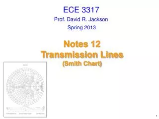
The Smith Chart (1) The Smith Chart represents the complex -plane within the unit circle. It is a conform mapping of the complex Z-plane onto itself using the transformation Imag(G) Imag(Z) Real(G) Real(Z) The real positive half plane of Z is thus transformed into the interior of the unit circle! Smith Chart
The Smith Chart (2) This is a “bilinear” transformation with the following properties: • generalized circles are transformed into generalized circles • circle circle • straight line circle • circle straight line • straight line straight line • angles are preserved locally a straight line is nothing else than a circle with infinite radius a circle is defined by 3 points a straight line is defined by 2 points Smith Chart
The Smith Chart (3) Impedances Z are usually first normalized by where Z0 is some characteristic impedance (e.g. 50 Ohm). The general form of the transformation can then be written as This mapping offers several practical advantages: 1. The diagram includes all “passive” impedances, i.e. those with positive real part, from zero to infinity in a handy format. Impedances with negative real part (“active device”, e.g. reflection amplifiers) would be outside the (normal) Smith chart. 2. The mapping converts impedances or admintances into reflection factors and vice-versa. This is particularly interesting for studies in the radiofrequency and microwave domain where electrical quantities are usually expressed in terms of “direct” or “forward” waves and “reflected” or “backward” waves. This replaces the notation in terms of currents and voltages used at lower frequencies. Also the reference plane can be moved very easily using the Smith chart. Smith Chart
The Smith Chart (4) The Smith Chart (Abaque Smith in French) is the linear representation of the complex reflection factor This is the ratio between backward and forward wave (implied forward wave a=1) i.e. the ratio backward/forward wave. The upper half of the Smith-Chart is “inductive” = positive imaginary part of impedance, the lower half is “capacitive” = negative imaginary part. Smith Chart
Important points Imag(G) Short Circuit Important Points: Short Circuit G = -1, z = 0 Open Circuit G = 1, z ® ¥ Matched Load G = 0, z = 1 On circle G = 1 lossless element Outside circle G = 1 active element, for instance tunnel diode reflection amplifier Open Circuit Real(G) MatchedLoad Smith Chart
The Smith Chart (5) 3. The distance from the center of the diagram is directly proportional to the magnitude of the reflection factor. In particular, the perimeter of the diagram represents full reflection, ||=1. Problems of matching are clearly visualize. Power into the load = forward power – reflected power max source power “(mismatch)” loss Here the US notion is used, where power = |a|2.European notation (often): power = |a|2/2These conventions have no impact on S parameters, only relevant for absolute power calculation Smith Chart
The Smith Chart (6) 4. The transition impedance admittance and vice-versa is particularly easy. Impedance z Reflection Admittance 1/z Reflection - Smith Chart
Navigation in the Smith Chart (1) in blue: Impedance plane (=Z) in red: Admittance plane (=Y) Series L Shunt L Shunt C Series C Navigation in the Smith Chart
Navigation in the Smith Chart (2) G R Toward load Toward generator Navigation in the Smith Chart
Impedance transformation by transmission lines The S-matrix for an ideal, lossless transmission line of length l is given by where is the propagation coefficient with the wavelength (this refers to the wavelength on the line containing some dielectric). N.B.: It is supposed that the reflection factors are evaluated with respect to the characteristic impedance Z0 of the line segment. How to remember that when adding a section of line we have to turn clockwise: assume we are at =-1 (short circuit) and add a very short piece of coaxial cable. Then we have made an inductance thus we are in the upper half of the Smith-Chart. Navigation in the Smith Chart
/4 - Line transformations Impedance z A transmission line of length transforms a load reflection load to its input as This means that normalized load impedance z is transformed into 1/z. In particular, a short circuit at one end is transformed into an open circuit at the other. This is the principle of /4-resonators. Impedance 1/z when adding a transmission line to some terminating impedance we move clockwise through the Smith-Chart. Navigation in the Smith Chart
Looking through a 2-port (1) In general: were in is the reflection coefficient when looking through the 2-port and load is the load reflection coefficient.The outer circle and the real axis in the simplified Smith diagram below are mapped to other circles and lines, as can be seen on the right. Line /16: 0 1 1 2 2 1 ¥ Attenuator 3dB: z = 0 z = ¥ ¥ 0 1 z = 1 or Z = 50 W Navigation in the Smith Chart
Looking through a 2-port (2) Lossless Passive Circuit 1 2 1 1 2 2 Lossy Passive Circuit Active Circuit Active Circuit: If potentially unstable If S is unitary Lossless Two-Port Lossy Two-Port: If unconditionally stable ¥ 0 1 0 0 1 1 ¥ Navigation in the Smith Chart ¥
Example: a Step in Characteristic Impedance (1) Consider a connection of two coaxial cables, one with ZC,1 = 50 characteristic impedance, the other with ZC,2 = 75 characteristic impedance. 2 1 Step 1: Calculate the reflection coefficient and keep in mind: all ports have to be terminated with their respective characteristic impedance, i.e. 75 for port 2. Thus, the voltage of the reflected wave at port 1 is 20% of the incident wave and the reflected power at port 1 (proportional 2) is 0.22 = 4%. As this junction is lossless, the transmitted power must be 96% (conservation of energy). From this we can deduce b22 = 0.96. But: how do we get the voltage of this outgoing wave? Connection between a 50 and a 75 cable. We assume an infinitely short cable length and just look at the junction. Example