Information criterion
Learn about likelihood calculation in Bayesian statistics for psychology. Explore examples, models, maximizing likelihood, and predicting log likelihood through practical exercises and simulations.


Information criterion
E N D
Presentation Transcript
Information criterion Greg Francis PSY 626: Bayesian Statistics for Psychological Science Fall 2018 Purdue University
Likelihood • Given a model (e.g., N(0, 1)), one can ask how likely is a set of observed data outcomes? • This is similar to probability, but not quite the same because in a continuous distribution, each specific point has probability zero • We multiply the probability density (height of model probability density function) of each data outcome • Smaller likelihoods indicate that data is less likely (probable), given the model X3 X1 X4 X2
Likelihood • Calculation is just multiplication of probability densities • > x<-c(-1.1, -0.3, 0.2, 1.0) • > dnorm(x, mean=0,sd=1) • [1] 0.2178522 0.3813878 0.3910427 0.2419707 • > prod(dnorm(x, mean=0,sd=1)) • [1] 0.007861686 X3 X1 X4 X2
Likelihood • It should be obvious that adding data to a set makes the set less likely • It is always more probable that I draw a red king from a deck of cards than that I draw a red king and then a black queen from a deck of cards. • x<-c(-1.1, -0.3, 0.2, 1.0, 0) • > prod(dnorm(x, mean=0,sd=1)) • [1] 0.003136359 • In general, larger data sets have smaller likelihood, for a given model • But this partly depends on the properties of the sets and the model X3 X5 X1 X4 X2
Log Likelihood • The values of likelihood can become so small that it causes problems • Smaller than the smallest possible number in a computer • Often compute log (natural) likelihood • > x<-c(-1.1, -0.3, 0.2, 1.0, 0) • > sum(dnorm(x, mean=0,sd=1, log=TRUE)) • [1] -5.764693 Smaller (more negative) values indicate smallerlikelihood X3 X5 X1 X4 X2
Maximum (log) Likelihood • Given a model (e.g., N(mu, 1)) form, what value of mu maximizes likelihood? • 0 -> -5.764693 • 0.5 -> -6.489693 • -0.5 -> -6.289693 • 0.05 -> -5.780943 • -0.05 -> -5.760943 • -0.025 -> -5.761255 • It is the sample mean -0.05 thatmaximizes (log) likelihood X3 X5 X1 X4 X2
Maximum (log) Likelihood • Given a model (e.g., N(mu, sigma)) form, what pair of parameters (mu, sigma) maximizes likelihood? • Sample standard deviation: (-0.05, 0.7635444) -> -5.246201 • Sample sd using “population formula” (-0.05, 0.6829348) -> -5.18845 • (-0.05, 0.5) -> -5.793957 • (-0.05, 1) -> -5.760943 • (0, 1) -> -5.764693 Note: the true population valuesdo not maximize likelihood for a given sample [Over fitting] X3 X5 X1 X4 X2
Predicting (log) Likelihood • Suppose you identify the parameters (e.g., N(mu, sigma)) that maximizes likelihood for a data set, X (n=50) • Now you gather a new data set Y (n=50). You use the (mu, sigma) values to estimate likelihood for the new data set • Repeat the process Average difference =1.54
Try again • Suppose you identify the parameters (e.g., N(mu, sigma)) that maximizes likelihood for a data set, X (n=50) • Now you gather a new data set Y (n=50). You use the (mu, sigma) values to estimate likelihood for the new data set Average difference =2.67
Really large sample • Suppose you identify the parameters (e.g., N(mu, sigma)) that maximizes likelihood for a data set, X (n=50) • Now you gather a new data set Y (n=50). You use the (mu, sigma) values to estimate likelihood for the new data set • Do this for many (100,000) simulated experiments and one finds (on average)
Different case • Suppose you identify the parameters (e.g., N(mu1, sigma), N(mu2, sigma)) that maximizes likelihood for a data set, X1, X2 (n1=n2=50) • Now you gather a new data set Y1, Y2 (n1=n2=50) • You use the (mu1, mu2, sigma) values to estimate likelihood for the new data set Average difference =2.68
Try again • Suppose you identify the parameters (e.g., N(mu1, sigma), N(mu2, sigma)) that maximizes likelihood for a data set, X1, X2 (n1=n2=50) • Now you gather a new data set Y1, Y2 (n1=n2=50) • You use the (mu1, mu2, sigma) values to estimate likelihood for the new data set Average difference =3.24
Really large sample • Suppose you identify the parameters (e.g., N(mu1, sigma), N(mu2, sigma)) that maximizes likelihood for a data set, X1, X2 (n1=n2=50) • Now you gather a new data set Y1, Y2 (n1=n2=50) • You use the (mu1, mu2, sigma) values to estimate likelihood for the new data set • Do this for many (100,000) simulated experiments and one finds (on average)
Still different case • Suppose you identify the parameters (e.g., N(mu1, sigma1), N(mu2, sigma2)) that maximizes likelihood for a data set, X1, X2 (n1=n2=50) • Now you gather a new data set Y1, Y2 (n1=n2=50) • You use the (mu1, mu2, sigma1, sigma2) values to estimate likelihood for the new data set • Do this for many (100,000) simulated experiments and one finds (on average)
Number of parameters • The difference of the log likelihood is approximately equal to the number of independent model parameters!
Over fitting • This means that, on average, the log likelihood of the original data set calculated relative to these parameter values is bigger than reality • It is a biased estimate of log likelihood • The log likelihood of the replication data set calculated relative to these parameter values is (on average) accurate • It is an unbiased estimate of log likelihood • Thus, we know that (on average) using the maximum likelihood estimates for parameters will “over fit” the data set • We can make a better estimate of the predicted likelihood of the original data set by adjusting for the (average) bias • Note, we only need to know how many (K) independent parameters are in the model • We do not actually need the replication data set!
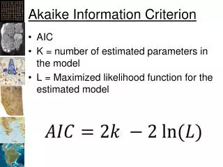
AIC • This is one way of deriving the Akaike Information Criterion • Multiply everything by -2 • More generally, AIC is an estimate of how much relative information is lost by using a model rather than (an unknown) reality • You can compare models by calculating AIC for each model (relative to a fixed data set) and choosing the model with the smaller AIC value • Learn how to pronounce his name • https://www.youtube.com/watch?v=WaiqX7JN4pI
Model comparison • Sample X and Y from N(0,1) and N(0.5, 1) for n1=n2=50
Model comparison • If you have to pick one model: Pick the one with the smallest AIC
Model comparison • How much confidence should you have in your choice? • Two steps:
Akaike weights • How much confidence should you have in your choice? • Two steps: • 1) Compute the difference of AIC, relative to the value of the best model
Akaike weights • How much confidence should you have in your choice? • Two steps: • 1) Compute the difference of AIC, relative to the value of the best model • 2) Rescale the differences to be a probability
Akaike weights • These are estimated probabilities that the given model will make the best predictions (of likelihood) on new data, conditional on the set of models being considered.
Generalization • AIC counts the number of independent parameters in the model • This is an estimate of the “flexibility” of the model to fit data • AIC works with the single “best” (maximum likelihood) parameters • In contrast, our Bayesian analyses consider a distribution of parameter values rather than a single “best” set • We can compute log likelihood for each set of parameter values in the posterior distribution • Average across them all (weighting by probability density) • WAIC (Widely Applicable Information Criterion) • Easy with the brms library • WAIC(model1) • Easy to compare models • WAIC(model1, model2, model3) > WAIC(model1, model2, model3) WAIC SE model1 691.87 13.14 model2 542.72 8.14 model3 550.11 9.55 model1 - model2 149.15 12.84 model1 - model3 141.76 11.64 model2 - model3 -7.39 4.67
Akaike weights • Easy with brms library • If you don’t like the scientific notation, try • Strongly favors model2, compared to the other choices here > model_weights(model1, model2, model3, weights="waic") model1 model2 model3 3.996742e-33 9.757196e-01 2.428036e-02 > options(scipen=999) > model_weights(model1, model2, model3, weights="waic") model1 model2 0.000000000000000000000000000000003996742 0.975719636846552385023301212640944868326 model3 0.024280363153447667018403066663267964032
loo vs. AIC • They are estimates of the same kind of thing: • Model complexity minus log likelihood • Asymptotically, AIC is an approximation of loo • AIC (and WAIC) is often easier/faster to compute than loo • In recent years, new methods for computing loo have been found, so some people recommend using loo whenever possible • You can compute the same kind of probability weights with loo > model_weights(model1, model2, model3, weights="loo") model1 model2 0.0000000000000000000000000000006490514 0.9723974775840951156880009875749237835 model3 0.0276025224159049606398319554045883706
Example: Visual Search • Typical results: For conjunctive distractors, response time increases with the number of distractors
Visual Search # Null model: no difference in slopes or intercepts model1 = brm(RT_ms ~ NumberDistractors, data = VSdata2, iter = 2000, warmup = 200, chains = 3, thin = 2 ) # print out summary of model print(summary(model1)) Family: gaussian Links: mu = identity; sigma = identity Formula: RT_ms ~ NumberDistractors Data: VSdata2 (Number of observations: 40) Samples: 3 chains, each with iter = 2000; warmup = 200; thin = 2; total post-warmup samples = 2700 Population-Level Effects: Estimate Est.Error l-95% CI u-95% CI Eff.Sample Rhat Intercept 835.56 172.88 502.72 1191.78 2441 1.00 NumberDistractors 32.50 4.72 23.01 41.58 2146 1.00 Family Specific Parameters: Estimate Est.Error l-95% CI u-95% CI Eff.Sample Rhat sigma 661.78 76.60 530.54 829.53 2145 1.00 • Let’s consider the effect of number of distractors and target being present or absent • Many different models • VSdata2<-subset(VSdata, VSdata$Participant=="Francis200S16-2" & VSdata$DistractorType=="Conjunction”) • Null model
# Model with a common intercept but different slopes for each condition model2 <- brm(RT_ms ~ Target:NumberDistractors, data = VSdata2, iter = 2000, warmup = 200, chains = 3) # print out summary of model print(summary(model2)) Family: gaussian Links: mu = identity; sigma = identity Formula: RT_ms ~ Target:NumberDistractors Data: VSdata2 (Number of observations: 40) Samples: 3 chains, each with iter = 2000; warmup = 200; thin = 1; total post-warmup samples = 5400 Population-Level Effects: Estimate Est.Error l-95% CI u-95% CI Eff.Sample Rhat Intercept 837.67 150.94 550.91 1135.34 4363 1.00 TargetAbsent:NumberDistractors 41.17 4.87 31.56 50.79 4621 1.00 TargetPresent:NumberDistractors 23.76 4.90 14.06 33.32 4061 1.00 Family Specific Parameters: Estimate Est.Error l-95% CI u-95% CI Eff.Sample Rhat sigma 579.46 69.13 459.84 736.52 4087 1.00 Visual Search • Let’s consider the effect of number of distractors and target being present or absent • Many different models • Different slopes
Visual Search # Model with different slopes and intercepts for each condition model3 <- brm(RT_ms ~ Target*NumberDistractors, data = VSdata2, iter = 2000, warmup = 200, chains = 3) # print out summary of model print(summary(model3)) Family: gaussian Links: mu = identity; sigma = identity Formula: RT_ms ~ Target * NumberDistractors Data: VSdata2 (Number of observations: 40) Samples: 3 chains, each with iter = 2000; warmup = 200; thin = 1; total post-warmup samples = 5400 Population-Level Effects: Estimate Est.Error l-95% CI u-95% CI Eff.Sample Rhat Intercept 832.81 215.85 407.45 1250.95 2830 1.00 TargetPresent 3.08 309.01 -596.13 605.03 2426 1.00 NumberDistractors 41.26 5.91 29.54 52.91 2742 1.00 TargetPresent:NumberDistractors -17.41 8.39 -34.09 -0.78 2276 1.00 Family Specific Parameters: Estimate Est.Error l-95% CI u-95% CI Eff.Sample Rhat sigma 588.64 71.71 470.35 747.28 4327 1.00 • Let’s consider the effect of number of distractors and target being present or absent • Many different models • Different slopes and different intercepts
Visual Search # Build a model using an exgaussian rather than a gaussian (better for response times) model4 <- brm(RT_ms ~ Target*NumberDistractors, family = exgaussian(link = "identity"), data = VSdata2, iter = 8000, warmup = 2000, chains = 3) # print out summary of model print(summary(model4)) Family: exgaussian Links: mu = identity; sigma = identity; beta = identity Formula: RT_ms ~ Target * NumberDistractors Data: VSdata2 (Number of observations: 40) Samples: 3 chains, each with iter = 8000; warmup = 2000; thin = 1; total post-warmup samples = 18000 Population-Level Effects: Estimate Est.Error l-95% CI u-95% CI Eff.Sample Rhat Intercept 828.08 210.69 414.36 1240.71 2285 1.00 TargetPresent 16.62 295.69 -561.13 587.66 1410 1.00 NumberDistractors 41.33 5.78 29.86 52.55 2427 1.00 TargetPresent:NumberDistractors -17.76 8.14 -33.48 -1.43 1660 1.00 Family Specific Parameters: Estimate Est.Error l-95% CI u-95% CI Eff.Sample Rhat sigma 576.34 66.46 464.18 722.07 5722 1.00 beta 25.73 10.24 14.75 53.92 1606 1.00 • Let’s consider the effect of number of distractors and target being present or absent • Many different models • Different slopes and different intercepts, exgaussian rather than gaussian
Visual Search • Compare models • Favors model2: common intercept, different slopes • But the data is not overwhelmingly in support of model2 • model3 and model4 might be viable too > model_weights(model1, model2, model3, model4, weights="waic") model1 model2 model3 model4 0.007507569 0.520042187 0.221238638 0.251211605 > model_weights(model1, model2, model3, model4, weights="loo") model1 model2 model3 model4 0.008902075 0.549701567 0.218741177 0.222655181
Serial search model • A popular theory about reaction times in visual search is that they are the result of a serial process • Examine an item and judge whether it is the target (green, circle) • If it is the target, then stop • If not, pick a new target and repeat • The final RT is determined (roughly) by how many items you have to examine before finding the target • When the target is present, on average you should find the target after examining half of the searched items • When the target is absent, you always have to search all the items • Thus slope(target absent) = 2 x slope(target present) • Is this a better model than just estimating each slope separately? • This twice slope model has less flexibility than the separate slopes model
Visual Search # A model where the slope for target absent is twice that for target present model5 <- brm(bf( RT_ms ~ a1 + b1*TargetIsPresent*NumberDistractors + 2*b1*(1-TargetIsPresent)*NumberDistractors, a1 ~1, b1 ~ 1, nl=TRUE), family = gaussian(),data = VSdata2, prior= c( prior(normal(0, 2000), nlpar="a1"), prior(normal(0, 300), nlpar="b1") ), iter = 8000, warmup = 2000, chains = 3) print(summary(model5)) Family: gaussian Links: mu = identity; sigma = identity Formula: RT_ms ~ a1 + b1 * TargetIsPresent * NumberDistractors + 2 * b1 * (1 - TargetIsPresent) * NumberDistractors a1 ~ 1 b1 ~ 1 Data: VSdata2 (Number of observations: 40) Samples: 3 chains, each with iter = 8000; warmup = 2000; thin = 1; total post-warmup samples = 18000 Population-Level Effects: Estimate Est.Error l-95% CI u-95% CI Eff.Sample Rhat a1_Intercept 878.41 140.82 601.19 1159.16 8065 1.00 b1_Intercept 20.76 2.42 15.99 25.52 8362 1.00 Family Specific Parameters: Estimate Est.Error l-95% CI u-95% CI Eff.Sample Rhat sigma 577.28 67.99 461.80 725.43 10473 1.00 • We have to tweak brms a bit to define this kind of model • There might be better ways to do what I am about to do • Define a dummy variable with value 0 if target is absent and 1 if the target is present • VSdata2$TargetIsPresent <- ifelse(VSdata2$Target=="Present", 1, 0) • We use the brm non-linear formula (even though we actually define a linear model)
Visual Search • Compare model2 (common intercept different slopes) and model5 (common intercept, twice-slopes) > WAIC(model2, model5) WAIC SE model2 627.47 11.55 model5 624.24 11.83 model2 - model5 3.23 2.55 > model_weights(model2, model5, weights="waic") model2 model5 0.165736 0.834264 > loo(model2, model5) LOOIC SE model2 627.86 11.73 model5 624.31 11.88 model2 - model5 3.55 2.59 > model_weights(model2, model5, weights="loo") model2 model5 0.1451945 0.8548055
> WAIC(model2, model5) WAIC SE model2 627.47 11.55 model5 624.24 11.83 model2 - model5 3.23 2.55 > model_weights(model2, model5, weights="waic") model2 model5 0.165736 0.834264 Visual Search • The twice-slope model has a smaller WAIC / loo, so it is expected to do a better job predicting future data than the more general separate slopes model • The theoretical constraint improves the model • Or, the extra parameter of the separate slopes model causes that model to over fit the sampled data, which hurts prediction of future data • How confident are we in this conclusion? • The Akaike weight is 0.83 for the twice-slope model • Pretty convincing, but maybe we hold out some hope for the more general model • Remember, the WAIC / loo values are estimates
# A model where the slope for target present is some multiple of the slope for target present (prior centered on 2) model6 <- brm(bf( RT_ms ~ a1 + b1*TargetIsPresent*NumberDistractors + b2*b1*(1-TargetIsPresent)*NumberDistractors, a1 ~1, b1 ~ 1, b2 ~1, nl=TRUE), family = gaussian(),data = VSdata2, prior= c( prior(normal(0, 2000), nlpar="a1"), prior(normal(0, 300), nlpar="b1"), prior(normal(2, 1), nlpar="b2")), iter = 8000, warmup = 2000, chains = 3) print(summary(model6)) Family: gaussian Links: mu = identity; sigma = identity Formula: RT_ms ~ a1 + b1 * TargetIsPresent * NumberDistractors + b2 * b1 * (1 - TargetIsPresent) * NumberDistractors a1 ~ 1 b1 ~ 1 b2 ~ 1 Data: VSdata2 (Number of observations: 40) Samples: 3 chains, each with iter = 8000; warmup = 2000; thin = 1; total post-warmup samples = 18000 Population-Level Effects: Estimate Est.Error l-95% CI u-95% CI Eff.Sample Rhat a1_Intercept 856.97 149.57 561.57 1146.31 9736 1.00 b1_Intercept 22.84 4.63 13.96 32.13 7736 1.00 b2_Intercept 1.85 0.36 1.30 2.70 7563 1.00 Family Specific Parameters: Estimate Est.Error l-95% CI u-95% CI Eff.Sample Rhat sigma 579.64 69.44 464.16 735.10 11024 1.00 Visual Search • Are we confident that the twice-slope model is appropriate? • Surely something like 1.9 x slope would work? • Why not put a prior on the multiplier?
Visual Search • Compare model5 (common intercept, twice-slope) and model6 (common intercept, variable slope multiplier) • Favors model5 (more specific slope) > WAIC(model5, model6) WAIC SE model5 624.24 11.83 model6 627.05 11.71 model5 - model6 -2.81 1.92 > model_weights(model5, model6, weights="waic") model5 model6 0.8030117 0.1969883 > loo(model5, model6) LOOIC SE model5 624.31 11.88 model6 627.43 11.92 model5 - model6 -3.11 1.94 > model_weights(model5, model6, weights="loo") model5 model6 0.8256974 0.1743026
Generalize serial search model • If final RT is determined (roughly) by how many items you have to examine before finding the target, then • When the target is present, on average you should find the target after examining half of the searched items • When the target is absent, you always have to search all the items • Thus slope(target absent) = 2 x slope(target present) • If this model were correct, then there should also be differences in standard deviations for Target present and Target absent trials • Target absent trials always have to search all the items (small variability) • Target present trials sometimes search all items, sometimes only search one item (and cases in between) (high variability)
Visual Search # A model where the slope for target absent is twice that for target present, and different variances for target conditions model7 <- brm(bf( RT_ms ~ a1 + b1*TargetIsPresent*NumberDistractors + 2*b1*(1-TargetIsPresent)*NumberDistractors, a1 ~1, b1 ~ 1, sigma ~ TargetIsPresent, nl=TRUE), family = gaussian(),data = VSdata2, prior= c( prior(normal(0, 2000), nlpar="a1"), prior(normal(0, 300), nlpar="b1") ), iter = 8000, warmup = 2000, chains = 3) print(summary(model7)) Family: gaussian Links: mu = identity; sigma = log Formula: RT_ms ~ a1 + b1 * TargetIsPresent * NumberDistractors + 2 * b1 * (1 - TargetIsPresent) * NumberDistractors a1 ~ 1 b1 ~ 1 sigma ~ TargetIsPresent Data: VSdata2 (Number of observations: 40) Samples: 3 chains, each with iter = 8000; warmup = 2000; thin = 1; total post-warmup samples = 18000 Population-Level Effects: Estimate Est.Error l-95% CI u-95% CI Eff.Sample Rhat sigma_Intercept 5.87 0.17 5.57 6.23 12599 1.00 a1_Intercept 856.75 113.51 634.23 1080.46 8825 1.00 b1_Intercept 20.62 1.67 17.34 23.93 8919 1.00 sigma_TargetIsPresent 0.71 0.23 0.25 1.17 14581 1.00 • We have to tweak brms a bit to define this kind of model • There might be better ways to do what I am about to do • Define a dummy variable with value 0 if target is absent and 1 if the target is present • VSdata2$TargetIsPresent <- ifelse(VSdata2$Target=="Present", 1, 0) • We use the brm non-linear formula (even though we actually define a linear model) • Include a function for sigma
Model comparison > WAIC(model5, model7) WAIC SE model5 624.24 11.83 model7 615.68 10.14 model5 - model7 8.55 5.23 > model_weights(model5, model7, weights="waic") model5 model7 0.01371064 0.98628936 > loo(model5, model7) LOOIC SE model5 624.31 11.88 model7 615.93 10.24 model5 - model7 8.38 5.24 > model_weights(model5, model7, weights="loo") model5 model7 0.01489884 0.98510116 • The twice-slope model with separate sd’s has the smallest WAIC / loo • The increased flexibility improves the model fit • The constraint on the twice-slope model to have a common sd, causes that model to under fit the data • How confident are we in this conclusion? • The Akaike weight is 0.98 for the twice-slope model with separate sd’s • Pretty convincing, but maybe we hold out some hope for the other models • Remember, the WAIC / loo values are estimates
Compare them all! > WAIC(model1, model2, model3, model4, model5, model6, model7) WAIC SE model1 635.94 9.78 model2 627.47 11.55 model3 629.18 11.29 model4 628.92 11.71 model5 624.24 11.83 model6 627.05 11.71 model7 615.68 10.14 model1 - model2 8.48 10.13 model1 - model3 6.77 10.00 model1 - model4 7.02 10.35 model1 - model5 11.71 12.21 model1 - model6 8.90 10.71 model1 - model7 20.26 11.25 model2 - model3 -1.71 0.31 model2 - model4 -1.46 0.28 model2 - model5 3.23 2.55 model2 - model6 0.42 0.66 model2 - model7 11.78 5.44 model3 - model4 0.25 0.45 model3 - model5 4.94 2.56 model3 - model6 2.13 0.77 model3 - model7 13.49 5.31 model4 - model5 4.69 2.42 model4 - model6 1.88 0.52 model4 - model7 13.24 5.47 model5 - model6 -2.81 1.92 model5 - model7 8.55 5.23 model6 - model7 11.36 5.38 > loo(model1, model2, model3, model4, model5, model6, model7) LOOIC SE model1 636.11 9.85 model2 627.86 11.73 model3 629.70 11.58 model4 629.67 12.17 model5 624.31 11.88 model6 627.43 11.92 model7 615.93 10.24 model1 - model2 8.25 10.27 model1 - model3 6.40 10.26 model1 - model4 6.44 10.75 model1 - model5 11.79 12.29 model1 - model6 8.68 10.90 model1 - model7 20.17 11.37 model2 - model3 -1.84 0.27 model2 - model4 -1.81 0.57 model2 - model5 3.55 2.59 model2 - model6 0.43 0.71 model2 - model7 11.93 5.55 model3 - model4 0.04 0.62 model3 - model5 5.39 2.52 model3 - model6 2.28 0.71 model3 - model7 13.77 5.47 model4 - model5 5.35 2.42 model4 - model6 2.24 0.55 model4 - model7 13.74 5.75 model5 - model6 -3.11 1.94 model5 - model7 8.38 5.24 model6 - model7 11.49 5.50 > model_weights(model1, model2, model3, model4, model5, model6, model7, weights="waic") model1 model2 model3 model4 model5 model6 model7 0.00003898635 0.00270054747 0.00114887880 0.00130452660 0.01359372494 0.00333470113 0.97787863471 > model_weights(model1, model2, model3, model4, model5, model6, model7, weights="loo") model1 model2 model3 model4 model5 model6 model7 0.00004066748 0.00251120979 0.00099927855 0.00101715895 0.01478427599 0.00312092166 0.97752648758
Generating models • It might be tempting to consider lots of other models • a model with separate slopes and separate sd’s • A model with twice slopes, separate sd’s and separate intercepts • All possibilities? • Different specific multipliers: 1.8, 1.9, 2.0, 2.1, 2.2, 2.3, 2.4,… • You should resist this temptation • There is always noise in your data, the (W)AIC / loo analysis hedges against over fitting that noise, but you can undermine it by searching for a model that happens to line up nicely with the particular noise in your sample • Models to test should be justified by some kind of argument • Theoretical processes involved in behavior • Previous findings in the literature • Practical implications
Model selection • Remember: If you have to pick one model: Pick the one with the smallest (W)AIC / loo • Consider whether you really have to pick just one model • If you want to predict performance on a visual search task, you will do somewhat better by merging the predictions of the different models instead of just choosing the best model • It is sometimes wise to just admit that the data do not distinguish between competing models, even if it slightly favors one • This can motivate future work • Do not make a choice unless you have to: • Such as, you are going to build a robot to search for targets • Even a clearly best model, is only relative to the set of models you have compared • There may be better models that you have not even considered because you did not gather the relevant information
Conclusions • Information Criterion • AIC relates number of parameters to differences of original and replication log likelihoods • WAIC generalizes the idea to more complex models (with posteriors of parameters) • It approximates loo, but is easier/faster to calculate • Can identify the best model that fits the data (maximizes log likelihood) with few parameters • Models should be justified • A more specific model is better, if it matches the data as well as a more general model