Linear Programming Models: Graphical and Computer Methods
Linear Programming Models: Graphical and Computer Methods. Chapter 7. Chapter Outline. 7.1 Introduction 7.2 Requirements of a Linear Programming Problem 7.3 Formulating LP Problems 7.4 Graphical Solution to an LP Problem 7.5 Solving LP Problem (QM for Window and Excel)

Linear Programming Models: Graphical and Computer Methods
E N D
Presentation Transcript
Linear Programming Models: Graphical and Computer Methods Chapter 7
Chapter Outline 7.1 Introduction 7.2 Requirements of a Linear Programming Problem 7.3 Formulating LP Problems 7.4 Graphical Solution to an LP Problem 7.5 Solving LP Problem (QM for Window and Excel) 7.6 Solving Minimization Problems 7.7 Four Special Cases in LP 7.8 Sensitivity Analysis
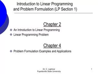
Linear Programming: An Overview • Objectives of business decisions frequently involve maximizing profit or minimizing costs. • Linear programming is an analytical technique in which linear algebraic relationships represent a firm’s decisions, given a business objective, and resource constraints. • Steps in application: • Identify problem as solvable by linear programming. • Formulate a mathematical model of the unstructured problem. • Solve the model. • Implementation
Requirements of LP Problems and LP Basic Assumptions Requirements • Decision variables- mathematical symbols representing levels of activity of a firm. • Objective function- a linear mathematical relationship describing an objective of the firm, in terms of decision variables - this function is to be maximized or minimized. • Constraints– requirements or restrictions placed on the firm by the operating environment, stated in linear relationships of the decision variables. • Parameters- numerical coefficients and constants used in the objective function and constraints. Assumptions • Proportionality - The rate of change (slope) of the objective function and constraint equations is constant. • Additivity- Terms in the objective function and constraint equations must be additive. • Divisibility -Decision variables can take on any fractional value and are therefore continuous as opposed to integer in nature. • Certainty - Values of all the model parameters are assumed to be known with certainty (non-probabilistic). • Non-negativity - all answers or variables are greater than or equal to (≥) zero
Pho (40K VND/bowl) Hu tieu (50K VND/bowl) Minime Restaurant Meat (120 grs meat/day) Chef (works 40 min./day) I can prepare 1 bowl of: - Pho in 1 min. - Hu tieu in 2 min. 1 bowl of: - Pho needs 4 gr meat - Hu tieu neads 3 gr. meat
LP Model Formulation A Maximization Example (1 of 3) • Product mix problem – Minime Noodle Restaurant How many bowls of Pho and Hu tieu should be prepared to maximize profits given labor and materials constraints? • Product resource requirements and unit profit:
LP Model Formulation A Maximization Example (2 of 3) • Trial and error • All for Pho: • 40 bowls 30 bowls 30 bowls x 40= 1200 (chef’s time surplus) • All for Hu tieu: • 20 bowls 40 bowls 20 bowls x 50= 1000 (meat surplus) • Half for Pho and Half for Hu tieu • PHO 20 bowls 15 bowls 15 bowls x 40= 600 (chef’s time surplus) • HU TIEU 10 bowls 20 bowls 10 bowls x 50= 500 (meat surplus) Time Meat Profit
LP Model Formulation A Maximization Example (3 of 3) Decision x1 = # of bowls of Pho to prepare per day Variables: x2 = # of bowls of Hu tieu to prepare per day ObjectiveMaximize Z = 40x1 + 50x2 Function:Where Z = profit per day subject to (s.t.): Resource 1x1 + 2x2 40 minutes of labor Constraints: 4x1 + 3x2 120 grs. of meat Non-Negativityx1 0; x2 0 Constraints:
Feasible and Infeasible Solutions • A feasible solution does not violate any of the constraints: Example x1 = 5 bowls of Pho x2 = 10 bowls of Hu tieu Z = 40x1 + 50x2 = 700 (K.VND) Labor constraint check: 1(5) + 2(10) = 25 < 40 minutes, within constraint Meat constraint check: 4(5) + 3(10) = 70 < 120 grams, within constraint • Aninfeasible solution violates at least one of the constraints: Example x1 = 10 bowls of Pho x2 = 20 bowls of Hu tieu • Z = 1400 (K.VND) Labor constraint check: 1(10) + 2(20) = 50 > 40 minutes, violates constraint
Graphical Solution of LP Models • Graphical solution is limited to linear programming models containing only two decision variables (can be used with three variables but only with great difficulty). • Graphical methods provide visualization of how a solution for a linear programming problem is obtained.
Coordinate Axes Graphical Solution of Maximization Model (1 of 11) Maximize Z = 40x1 + 50x2 subject to: 1x1 + 2x2 40 4x1 + 3x2 120 x1, x2 0 Figure 2.2 Coordinates for Graphical Analysis
Labor Constraint Graphical Solution of Maximization Model (2 of 11) Maximize Z = 40x1 + 50x2 subject to: 1x1 + 2x2 40 4x1 + 3x2 120 x1, x2 0 Figure 2.3 Graph of Labor Constraint
Labor Constraint Area Graphical Solution of Maximization Model (3 of 11) Maximize Z = 40x1 + 50x2 subject to: 1x1 + 2x2 40 4x1 + 3x2 120 x1, x2 0 Figure 2.4 Labor Constraint Area
Meat Constraint Area Graphical Solution of Maximization Model (4 of 11) Maximize Z = 40x1 + 50x2 subject to: 1x1 + 2x2 40 4x1 + 3x2 120 x1, x2 0 Figure 2.5 Clay Constraint Area
Both Constraints Graphical Solution of Maximization Model (5 of 11) Maximize Z = 40x1 + 50x2 subject to: 1x1 + 2x2 40 4x1 + 3x2 120 x1, x2 0 Figure 2.6 Graph of Both Model Constraints
Feasible Solution Area Graphical Solution of Maximization Model (6 of 11) Maximize Z = 40x1 + 50x2 subject to: 1x1 + 2x2 40 4x1 + 3x2 120 x1, x2 0 Figure 2.7 Feasible Solution Area
Isoprofit Line Method Graphical Solution of Maximization Model (7 of 11) Maximize Z = 40x1 + 50x2 subject to: 1x1 + 2x2 40 4x1 + 3x2 120 x1, x2 0 • Construct the isoprofit line: • Z = 40x1 + 50x2 • x2 = Z/50 - 40/50x1 = Z/50 -4/5x1 Figure 2.8 Objection Function Line for Z = $800
Isoprofit Line Method Graphical Solution of Maximization Model (8 of 11) Maximize Z = 40x1 + 50x2 subject to: 1x1 + 2x2 40 4x1 + 3x2 120 x1, x2 0 Figure 2.9 Alternative Objective Function Lines
Isoprofit Line Method Graphical Solution of Maximization Model (9 of 11) Maximize Z = 40x1 + 50x2 subject to: 1x1 + 2x2 40 4x1 + 3x2 120 x1, x2 0 Figure 2.10 Identification of Optimal Solution
Optimal Solution Coordinates Graphical Solution of Maximization Model (10 of 11) Maximize Z = 40x1 + 50x2 subject to: 1x1 + 2x2 40 4x1 + 3x2 120 x1, x2 0 Figure 2.11 Optimal Solution Coordinates
Extreme (Corner) Point Method Graphical Solution of Maximization Model (11 of 11) Maximize Z = 40x1 + 50x2 subject to: 1x1 + 2x2 40 4x1 + 3x2 120 x1, x2 0 Figure 2.12 Solutions at All Corner Points
Using Excel’s Solverto Solve LP Problems • The Solver tool in Excel can be used to find solutions to • LP problems • Integer programming problems • Noninteger programming problems • Solver may be sensitive to the initial values it uses • Solver is limited to 200 variables and 100 constraints • It can be used for small real world problems • Add-ins like What’s Best! Can be used to expand Solver’s capabilities
Click on “Tools” to invoke “Solver.” Objective function =E6-F6 =E7-F7 =C6*B10+D6*B11 =C7*B10+D7*B11 Decision variables – Pho (x1)=B10; Hu tieu (x2)=B11 Using Excel’s Solverto Solve LP Problems Maximize Z = 40 x1 + 50 x2 Subject to x1 + 2x2 40 mins. (labor constraint) 4x1 + 3x2 120 grs. (meat constraint) x1 , x2 0
After all parameters and constraints have been input, click on “Solve.” Objective function Decision variables C6*B10+D6*B11≤40 C7*B10+D7*B11≤120 Click on “Add” to insert constraints Using Excel’s Solver to Solve LP Problems
subject to 4T + 3C ≤ 240 (carpentry constraint) 2T + 1C ≤ 100 (painting and varnishing constraint) T, C≥ 0 (nonnegativity constraint) Using QM for Windows and Excel Solving Flair Furniture’s LP Problem • Most organizations have access to software to solve big LP problems • While there are differences between software implementations, the approach each takes towards handling LP is basically the same • Once you are experienced in dealing with computerized LP algorithms, you can easily adjust to minor changes Maximize profit = $70T + $50C
Using QM for Windows • First select the Linear Programming module • Specify the number of constraints (non-negativity is assumed) • Specify the number of decision variables • Specify whether the objective is to be maximized or minimized • For the Flair Furniture problem there are two constraints, two decision variables, and the objective is to maximize profit • Computer screen for input of data
Using QM for Windows • Computer screen for input of data • Computer screen for output of solution
Using QM for Windows • Graphical output of solution
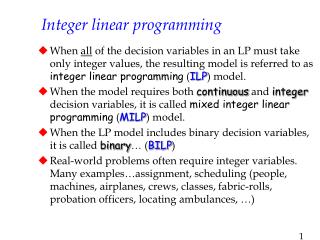
LP Model Formulation A Minimization Example (1 of 6) • Two brands of fertilizer available - Super-Gro, Crop-Quick. • Field requires at least 16 pounds of nitrogen and 24 pounds of phosphate. • Super-Gro costs $6 per bag, Crop-Quick$3 per bag. • Problem: How much of each brand to purchase to minimize total cost of fertilizer given following data ?
LP Model Formulation A Minimization Example (2 of 6) Decision Variables: x1 = bags of Super-Gro x2 = bags of Crop-Quick The Objective Function: Minimize Z = 6x1 + 3x2 Model Constraints: 2x1 + 4x2 16 lb (nitrogen constraint) 4x1 + 3x2 24 lb (phosphate constraint) x1, x2 0 (non-negativity constraint)
LP Model Formulation and Constraint Graph A Minimization Example (3 of 6) Minimize Z = $6x1 + $3x2 subject to: 2x1 + 4x2 16 4x1 + 3x2 24 x1, x2 0 Figure 2.16 Graph of Both Model Constraints
Feasible Solution Area A Minimization Example (4 of 6) Minimize Z = $6x1 + $3x2 subject to: 2x1 + 4x2 16 4x1 + 3x2 24 x1, x2 0 Figure 2.17 Feasible Solution Area
Optimal Solution Point A Minimization Example (5 of 6) Minimize Z = $6x1 + $3x2 subject to: 2x1 + 4x2 16 4x1 + 3x2 24 x1, x2 0 • Construct the objective line: • Z = 6x1 + 3x2 • x2 = Z/3 – 6/3x1 • x2 = Z/3 -2x1 Figure 2.18 Optimum Solution Point
Graphical Solutions A Minimization Example (6 of 6) Minimize Z = $6x1 + $3x2 subject to: 2x1 + 4x2 16 4x1 + 3x2 24 x1, x2 0 Figure 2.19 Graph of Fertilizer Example
Four Special Cases in LP • Four special cases and difficulties arise at times when using the graphical approach to solving LP problems • Infeasibility • Unboundedness • Redundancy • Alternate Optimal Solutions
X2 8 – – 6 – – 4 – – 2 – – 0 – Region Satisfying Third Constraint | | | | | | | | | | 2 4 6 8 X1 Four Special Cases in LP • Infeasibility-A problem with no feasible solution • Exists when there is no solution to the problem that satisfies all the constraint equations • No feasible solution region exists Region Satisfying First Two Constraints
X2 15 – 10 – 5 – 0 – | | | | | 5 10 15 X1 Four Special Cases in LP • Unboundedness- A solution region unbounded to the right • In a graphical solution, the feasible region will be open ended • This usually means the problem has been formulated improperly X1≥ 5 X2≤ 10 Feasible Region X1 + 2X2≥ 15
X2 30 – 25 – 20 – 15 – 10 – 5 – 0 – | | | | | | 5 10 15 20 25 30 X1 Four Special Cases in LP • Redundancy- A problem with a redundant constraint • A redundant constraint is one that does not affect the feasible solution region 2X1 + X2≤ 30 Redundant Constraint X1≤ 25 X1 + X2≤ 20 Feasible Region
X2 8 – 7 – 6 – 5 – 4 – 3 – 2 – 1 – 0 – A B | | | | | | | | 1 2 3 4 5 6 7 8 X1 Four Special Cases in LP • Alternate optimal solutions • Occasionally two or more optimal solutions may exist • Graphically this occurs when the objective function’s isoprofit or isocost line runs perfectly parallel to one of the constraints Optimal Solution Consists of All Combinations of X1 and X2 Along the AB Segment Isoprofit Line for $8 Isoprofit Line for $12 Overlays Line Segment AB Feasible Region
Sensitivity Analysis • Sensitivity analysis is used to determine effects on the optimal solution within specified ranges for the objective function coefficients, constraint coefficients, and right hand side (RHS) values. • Sensitivity analysis provides answers to certain what-if questions.
Range of Optimality • A range of optimality of an objective function coefficient is found by determining an interval for the objective function coefficient in which the original optimal solution remains optimal while keeping all other data of the problem constant. The value of the objective function may change in this range. • Graphically, the limits of a range of optimality are found by changing the slope of the objective function linewithin the limits of the slopes of the binding constraint lines. (This would also apply to simultaneous changes in the objective coefficients.) • The slope of an objective function line, Max c1x1 + c2x2, is -c1/c2 The slope of a constraint, a1x1 + a2x2 = b, is -a1/a2
Shadow Price • A shadow price for a RHS value (or resource limit) is the amount the objective function will change per unit increase in the right hand side value of a constraint. • Graphically, a shadow price is determined by adding +1 to the right hand side value in question and then resolving for the optimal solution in terms of the same two binding constraints. • The shadow price is equal to the difference in the values of the objective functions between the new and original problems. • The shadow price for a nonbinding constraint is 0.
Example: Sensitivity Analysis • Solve graphically for the optimal solution: Max z = 5x1 + 7x2 s.t. x1< 6 2x1 + 3x2< 19 x1 + x2< 8 x1, x2> 0
Example: Sensitivity Analysis • Graphical Solution x2 x1 + x2< 8 8 7 6 5 4 3 2 1 1 2 3 4 5 6 7 8 9 10 Max 5x1 + 7x2 x1< 6 Optimal x1 = 5, x2 = 3 z = 46 2x1 + 3x2< 19 x1
Example: Sensitivity Analysis • Range of Optimality for c1 The slope of the objective function line is-c1/c2. The slope of the 1st binding constraint, x1 + x2 = 8, is -1, the slope of the 2nd binding constraint, 2x1 + 3x2 = 19, is -2/3. Find the range of values for c1 (with c2 staying 7) such that the objective function line slope lies between that of the two binding constraints: -1 < -c1/7 < -2/3 Multiplying through by -7 (and reversing the inequalities): 14/3 <c1< 7
Example: Sensitivity Analysis • Range of Optimality for c2 Find the range of values for c2 ( with c1 staying 5) such that the objective function line slope lies between that of the two binding constraints: -1 < -5/c2< -2/3 Multiplying by -1: 1 > 5/c2> 2/3 Inverting, 1 <c2/5 < 3/2 Multiplying by 5: 5 <c2< 15/2
Example: Sensitivity Analysis • Shadow Prices Constraint 1: Since x1< 6 is not a binding constraint, its shadow price is 0. Constraint 2: Change the RHS value of the 2nd constraint to 20 and resolve for the optimal point determined by the last two constraints: 2x1 + 3x2 = 20 and x1 + x2 = 8. The solution is x1 = 4, x2 = 4, z = 48. Hence, the shadow price = znew - zold = 48 - 46 = 2. Constraint 3: Change the RHS value of the 3rd constraint to 9 and resolve for the optimal point determined by the last two constraints: 2x1 + 3x2 = 19 and x1 + x2 = 9. The solution is: x1 = 8, x2 = 1, z = 47. Hence, the shadow price = znew - zold = 47 - 46 = 1.