Interpolating Functions from Large Boolean Relations
Interpolating Functions from Large Boolean Relations. Jie-Hong Roland Jiang, Hsuan-Po Lin, and Wei-Lun Hung Grad. Inst. of Electronics Eng. / Dept of Electrical Eng. National Taiwan University. Outline. ◆ Introduction. ◆ Our Approach . ◆ Experimental Results. ◆ Conclusions.


Interpolating Functions from Large Boolean Relations
E N D
Presentation Transcript
Interpolating Functions from Large Boolean Relations Jie-Hong Roland Jiang, Hsuan-Po Lin, and Wei-Lun Hung Grad. Inst. of Electronics Eng. / Dept of Electrical Eng. National Taiwan University
Outline ◆ Introduction ◆ Our Approach ◆ Experimental Results ◆ Conclusions
Relations vs. Functions Boolean relation R(X, Y) Boolean function F(X) Disallow one-to-many mappings Can only describe deterministic behavior A special case of relation • Allow one-to-many mappings • Can describe non-deterministic behavior • More generic than functions x1x2 x1x2 y1y2 y1y2 00 00 00 00 01 01 01 01 10 10 10 10 11 11 11 11 f1 = x1 x2 f2 = x1 x2
Total Relations vs. Partial Relations Total relation Partial relation Some input element is not mapped to any output element • Every input element is mapped to at least one output element x1x2 y x1x2 y 00 00 0 0 01 01 10 10 1 1 11 11
Totalization • A partial relation can be totalized • Assume that the input element not mapped to any output element is a don’t care x1x2 y x1x2 y Total relation Partial relation 00 00 Totalize 0 0 01 01 10 10 1 1 11 11 T(X, y) = R(X, y) y. R(X, y)
Application of Boolean Relations • In high-level design, Boolean relations can be used to describe (nondeterministic) specifications • In gate-level design, Boolean relations can be used to characterize the flexibility of sub-circuits • Boolean relations are more powerful than traditional don’t-care representations x1x2 y1y2 00 00 01 01 10 10 11 11
Needs of Relation Determinization • For hardware implement of a system, we need functions rather than relations • Physical realization are deterministic by nature • One input stimulus results in one output response
Needs of Relation Determinization • To simplify implementation, we can explore the flexibilities described by a relation for optimization y1 y1 z1 x1 z1 x2 x2 x1 z2 z2 y2 y2 f1 = x1 x2 f2 = x1 x2 f1 = x2 f2 = x1 00 00 00 01 01 01 x1x2 y1y2 z1z2 10 10 10 11 11 11
Problem Statement • Given a nondeterministic Boolean relation R(X, Y), how to determinize and extract functions from it? • For a deterministic total relation, we can uniquely extract the corresponding functions
Related Work • Prior Work • BDD- or SOP-based representation • Not scalable • Focused on function optimization • Ours • AIG representation • Focus on scalability with reasonable optimization quality
Enabling Technique • Craig Interpolation Theorem • If φA φB is UNSAT for propositional formulas φA ,φB, • then there exists an interpolantI such that • φA→I • IφBis UNSAT • I refers only to the common • variables of φAand φB I φB φA
Single-Output Relations • For a single-output total relationR(X, y), we derive a function f for variable y using interpolation R(X,0) R(X,1) is UNSAT 11 00 10 x1x2 y 00 I 0 01 10 φA φB 1 11 φB : R(X,1) Minimal care offset of f φA : R(X,0) Minimal care onset of f
Interpolantion vs. Cofactoring • Naïve derivation of f is by cofactoring • R(X,1) (largest onset of f) or • R(X,0) (smallest onset of f) φB= R(X,1) Largest onset of f 00 11 10 x1x2 y φA= R(X,0) Smallest onset of f I 00 0 01 The function extracted from a single-output relation using cofactor is usually of similar size as the relation 10 φA φB 1 11 • Interpolation may extract smaller functions and prevent AIG explosion R(X,0) ⊆ I ⊆ R(X,1)
Multiple-Output Relations • Two-phase computation: • Phase 1 : Backward reduction • Reduce to single-output case R(X, y1, …, yn) →y2, …, yn. R(x, y1, …, yn) • Existential quantification using expansion y. φ(x,y) = φ(x,1) + φ(x,0) • Existential quantification using substitution [CAV 2009] y. φ(x,y) = φ(x, f(x)) • Phase 2 : Forward substitution • Extract functions
Multiple-Output Relations Example (Xp) R(3) R(2) R Phase1: (expansion reduction) y3.R(X, y1, y2 , y3) → R(3)(X, y1, y2) y2.R(3)(X, y1, y2) → R(2)(X, y1) y1 y2 y3 X Phase2: R(2)(X, y1) → y1 = f1(X) R(3)(X, y1, y2) → R(3)(X, f1(X), y2) → y2 = f2(X) R(X, y1, y2 , y3) → R(X, f1(X), f2(X), y2) → y3 = f3(X) f3 f2 f1 X X X
Multiple-Output Relations Example (St) R<3> R<2> R Phase1: (substitution reduction) R(X, y1, y2 , y3) → y3 = f3’(X , y1, y2 ) → R<3>(X, y1, y2) R<3>(X, y1, y2) → y2 = f2’(X , y1 ) → R<2>(X, y1) y1 y2 y3 X Phase2: R<2>(X, y1) → y1 = f1(X) R<3>(X, y1, y2) → R<3>(X, f1(X), y2) → y2 = f2(X) R(X, y1, y2 , y3) → R(X, f1(X), f2(X), y2) → y3 = f3(X) f2 f3 f1 f3' f2' X X X y1 y1 y2 X X
Multiple-Output Relations Example (SD) R<2> R<3> R Phase1: (substitution reduction) R(X, y1, y2 , y3) → y3 = f3’(X , y1, y2 ) → R<3>(X, y1, y2) R<3>(X, y1, y2) → y2 = f2’(X , y1 ) → R<2>(X, y1) R<2>(X, y1, y2) → y1 = f1’(X) y1 y2 y3 X Phase2: (interpolation for deterministic rel.) D = R Λ ∏i (yi ≡ fi’) fi(X) = Interpolant(Dyi, D yi) f1 f2 f3 f3' f2' f1' X X X y1 y1 y2 X X X
Experimental Setup • Our methods were implemented in ABC using MiniSAT • We prepare Boolean relations by computing the transition relations of ISCAS and ITC circuits • Insert don’t cares to introduce nondeterminism • Represent transition relations using AIGs
Experimental Results – w/o DC --- : BDD nodes are over 500K during computation
Experimental Results – w/ DC --- : BDD nodes are over 500K during computation
Experimental Results (cont’d) • Further synthesis by ABC commands “collapse” and “dc2”
Experimental Results (cont’d) • Interpolant vs. cofactor
Conclusions • Scalable function extraction from Boolean relations • Interpolation plays an essential role • Relations with up to thousands of variables can be determinized inexpensively • Extracted functions are of reasonable sizes • Future work • Determinization scheduling • Simple function extraction