Equalization
Equalization. Equalization. Fig. Digital communication system using an adaptive equaliser at the receiver. Equalization. Equalization compensates for or mitigates inter-symbol interference (ISI) created by multipaths in time dispersive channels (frequency selective fading channels).

Equalization
E N D
Presentation Transcript
Equalization Fig. Digital communication system using an adaptive equaliser at the receiver.
Equalization • Equalization compensates for or mitigates inter-symbol interference (ISI) created by multipaths in time dispersive channels (frequency selective fading channels). • Equalizer must be “adaptive”, since channels are time varying.
Zero forcing equalizer • Design from frequency domain viewpoint.
Zero forcing equalizer • ∴ must compensate for the channel distortion. ⇒ Inverse channel filter ⇒ completely eliminates ISI caused by the channel ⇒ Zero Forcing equaliser, ⇒ ZF.
Zero forcing equalizer Fig. Pulses having a raised cosine spectrum
Zero forcing equalizer • Example: A two-path channel with impulse response The transfer function is The inverse channel filter has the transfer function
Zero forcing equalizer • Since DSP is generally adopted for automatic equalizers ⇒ it is convenient to use discrete time (sampled) representation of signal. • Received signal • For simplicity, assume say
Zero forcing equalizer • Denote a T-time delay element by Z− 1, then
Zero forcing equalizer • The transfer function of the inverse channel filter is • This can be realized by a circuit known as the linear transversal filter.
Zero forcing equalizer • The exact ZF equalizer is of infinite length but usually implemented by a truncated (finite) length approximation. • For , a 2-tap version of the ZF equalizer has coefficients
Modeling of ISI channels • Complex envelope of any modulated signal can be expressed as where ha(t) is the amplitude shaping pulse.
Modeling of ISI channels • In general, ASK, PSK, and QAM are included, but most FSK waveforms are not. • Received complex envelope is where is channel impulse response. • Maximum likelihood receiver has impulse response matched to f(t)
Modeling of ISI channels • Output: • where nb(t) is output noise and
Least Mean Square Equalizers Fig. A basic equaliser during training
Least Mean Square Equalizers • Minimization of the mean square error (MSE), ⇒ MMSE. Equalizer input h(t): impulse response of tandem combination of transmit filter, channel and receiver filter. • In the absence of noise and ISI • The error due to noise and ISI at t=kT is given by • The error is
Least Mean Square Equalizers • The MSE is • In order to minimize , we require ……
Least Mean Square Equalizers • The optimum tap coefficients are obtained as W = R−1P. • But this is solved on the knowledge of xk's, which are the transmitted pilot data. • A given sequence of xk's called a test signal, reference signal or training signal is transmitted prior to the information signal, (periodically). • By detecting the training sequence, the adaptive algorithm in the receiver is able to compute and update the optimum wnk‘s -- until the next training sequence is sent.
Least Mean Square Equalizers • Example: • Determine the tap coefficients of a 2-tap MMSE for: • Now, given that
Mean Square Error (MSE) for optimum weights • Now, the optimum weight vector was obtained as • Substituting this into the MSE formula above, we have
Mean Square Error (MSE) for optimum weights • Now, apply 3 matrix algebra rules: • For any square matrix • For any matrix product • For any square matrix
Mean Square Error (MSE) for optimum weights • For the example
MSE for zero forcing equalizers • Recall for ZF equalizer • Assuming the same channel and noise as for the MMSE equalizer for MMSE
MSE for zero forcing equalizers • The ZF equalizer is an inverse filter; ⇒ it amplifies noise at frequencies where the channel transfer function has high attenuation. • The LMS algorithm tends to find optimum tap coefficients compromising between the effects of ISI and noise power increase, while the ZF equalizer design does not take noise into account.
Diversity Techniques • Mitigates fading effects by using multiple received signals which experienced different fading conditions. • Space diversity: With multiple antennas. • Polarization diversity: Using differently polarized waves. • Frequency diversity: With multiple frequencies. • Time diversity: By transmission of the same signal in different times. • Angle diversity: Using directive antenna aimed at different directions. • Signal combining methods. • Maximal Ratio combining.
Diversity Techniques • Equal gain combining. • Selection (switching) combining. • Space diversity is classified into micro-diversity and macro-diversity. • Micro-diversity: Antennas are spaced closely to the order of a wavelength. Effective for fast fading where signal fades in a distance of the order of a wavelength. • Macro (site) diversity: Antennas are spaced wide enough to cope with the topographical conditions ( eg: buildings, roads, terrain). Effective for shadowing, where signal fades due to the topographical obstructions.
PDF of SNR for diversity systems • Consider an M-branch space diversity system. • Signal received at each branch has Rayleigh distribution. • All branch signals are independent of one another. • Assume the same mean signal and noise power ⇒ the same mean SNR for all branches. • Instantaneous
PDF of SNR for diversity systems • Probability that takes values less than some threshold x is,
Selection Diversity • Branch selection unit selects the branch that has the largest SNR. • Events in which the selector output SNR, , is less than some value, x,is exactly the set of events in which each is simultaneously below x. • Since independent fading is assumed in each of the M branches,
Maximal Ratio Combining • is complex envelope of signal in the k-th branch. • The complex equivalent low-pass signal u(t) containing the information is common to all branches. • Assume u(t) normalized to unit mean square envelope such that
Maximal Ratio Combining • Assume time variation of gk (t) is much slower than that of u(t) . • Let nk(t) be the complex envelope of the additive Gaussian noise in the k-th receiver (branch). ⇒ usually all k N are equal.
Maximal Ratio Combining • Now define SNR of k-th branch as • Now, • Where are the complex combining weight factors. • These factors are changed from instant to instant as the branch signals change over the short term fading.
Maximal Ratio Combining • These factors are changed from instant to instant as the branch signals change over the short term fading. • How should be chosen to achieve maximum combiner output SNR at each instant? • Assuming nk(t)’s are mutually independent (uncorrelated), we have
Maximal Ratio Combining • Instantaneous output SNR, ,
Maximal Ratio Combining • Apply the Schwarz Inequality for complex valued numbers. • The equality holds if for all k, where K is an arbitrary complex constant. • Let
Maximal Ratio Combining with equality holding if and only if , for each k. • Optimum weight for each branch has magnitude proportional to the signal magnitude and inversely proportional to the branch noise power level, and has a phase, canceling out the signal (channel ) phase. • This phase alignment allows coherent addition of branch signals ⇒“co-phasing”.
Maximal Ratio Combining each has a chi-square distribution. • is distributed as chi-square with 2M degrees of freedom. • Average SNR, , is simply the sum of the individual • for each branch, which is Γ,
Convolutional CodesDepartment of Electrical EngineeringWang Jin
Overview • Background • Definition • Speciality • An Example • State Diagram • Code Trellis • Transfer Function • Summary • Assignment
Background • Convolutional code is a kind of code using in digital communication systems • Using in additive white Gaussian noise channel • To improve the performance of radio and satellite communication systems • Include two parts: encoding and decoding
Block codes Vs Convolutional Codes • Block codes take k input bits and produce n output bits, where kand nare large • There is no data dependency between blocks • Useful for data communications • Convolution codes take a small number of input bits and produce a small number of output bits each time period • Data passes through convolutional codes in a continuous stream • Useful for low-latency communication