Download
1 / 8
80 likes | 252 Vues
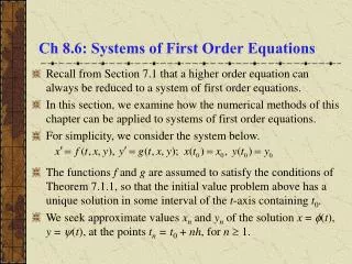
Ch 8.6: Systems of First Order Equations. Recall from Section 7.1 that a higher order equation can always be reduced to a system of first order equations. In this section, we examine how the numerical methods of this chapter can be applied to systems of first order equations.

E N D
Ch 8.6: Systems of First Order Equations • Recall from Section 7.1 that a higher order equation can always be reduced to a system of first order equations. • In this section, we examine how the numerical methods of this chapter can be applied to systems of first order equations. • For simplicity, we consider the system below. • The functions f and g are assumed to satisfy the conditions of Theorem 7.1.1, so that the initial value problem above has a unique solution in some interval of the t-axis containing t0. • We seek approximate values xn and yn of the solution x = (t), y = (t), at the points tn = t0 + nh, for n 1.
Vector Notation • In vector notation, the initial value problem can be written as where • The numerical methods of the previous sections can be readily generalized to handle systems of two or more equations. • To accomplish this, we simply replace x and f in the numerical formulas with x and f, as illustrated in the following slides.
Euler Method • Recall the Euler method for a uniform step size h: • In vector notation, this can be written as or • The initial conditions are used to determine f0, the tangent vector to the graph of the solution x = (t) in the xy-plane. • We move in the direction of this tangent vector f0 for a time step h in order to find x1, then find a new tangent vector f1, move along it for a time step h in order to find x2, and so on.
Runge-Kutta Method • In a similar way, the Runge-Kutta method can be extended to a system of equations. The vector formula is given by where • To help better understand the notation here, observe that
Example 1: Exact Solution (1 of 4) • Consider the initial value problem • We will use Euler’s method with h = 0.1 and the Runge-Kutta method with h = 0.2 to approximate the solution at t = 0.2, and then compare results with the exact solution: • For this problem, note that fn = xn-4yn and gn = - xn+ yn, and that f and g are independent of t, with
Example 1: Euler Method (2 of 4) • We have x0 = 1, y0 = 0, and • Using the Euler formulas with h = 0.1, • The values of the exact solution, correct to eight digits, are • Thus the Euler method approximation errors are 0.0704 and 0.0308, respectively, with corresponding relative errors of about 5.3% and 12.3%.
Example 1: Runge-Kutta Method (3 of 4) • Using the Runge-Kutta formulas for kni, and recalling that x0 = 1, y0 = 0, we obtain, for h = 0.2, • The errors for x1 and y1 are .000358 and .000180, respectively, with relative errors of about 0.0271% and 0.072%.
Example 1: Summary (4 of 4) • This example again illustrates the great gains in accuracy that are possible by using a more accurate approximation method, such as the Runge-Kutta method. • In the calculations for this example, the Runge-Kutta method requires only twice as many function evaluations as the Euler method, but the error in the Runge-Kutta method is about 200 times less than in the Euler method.