Bias-Variance in Machine Learning: A Detailed Overview
460 likes | 692 Vues
Explore the concepts of bias and variance, underfitting, overfitting, and error in machine learning. Learn how to measure, reduce error, and apply bias-variance decomposition in regression and classification. Discover practical examples and methods using synthetic data.

Bias-Variance in Machine Learning: A Detailed Overview
E N D
Presentation Transcript
Bias-Variance: Outline • Underfitting/overfitting: • Why are complex hypotheses bad? • Simple example of bias/variance • Error as bias+variance for regression • brief comments on how it extends to classification • Measuring bias, variance and error • Bagging - a way to reduce variance • Bias-variance for classification
Bias/Variance is a Way to UnderstandOverfitting and Underfitting high error “too simple” “too complex” Error/Loss on an unseen test set Dtest Error/Loss on training set Dtrain complex classifier simple classifier 3
Example Tom Dietterich, Oregon St
Example Tom Dietterich, Oregon St Same experiment, repeated: with 50 samples of 20 points each
noise is similar to error1 The true function f can’t be fit perfectly with hypotheses from our class H (lines) Error1 Fix: more expressive set of hypotheses H We don’t get the best hypothesis from H because of noise/small sample size Error2 Fix: less expressive set of hypotheses H
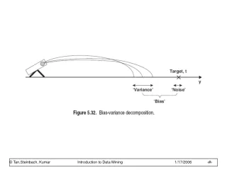
Bias and variance for regression • For regression, we can easily decompose the error of the learned model into two parts: bias (error 1) and variance (error 2) • Bias: the class of models can’t fit the data. • Fix: a more expressive model class. • Variance: the class of models could fit the data, but doesn’t because it’s hard to fit. • Fix: a less expressive model class.
Bias – Variance decomposition of error learned from D dataset and noise true function noise Fix test case x, then do this experiment: 1. Draw size n sample D=(x1,y1),….(xn,yn) 2. Train linear regressor hD using D 3. Draw one test example (x, f(x)+ε) 4. Measure squared error of hD on that example x What’s the expected error?
Bias – Variance decomposition of error Notation - to simplify this learned from D dataset and noise true function noise long-term expectation of learner’s prediction on this x averaged over many data sets D
Bias – Variance decomposition of error VARIANCE Squared difference between best possible prediction for x, f(x), and our “long-term” expectation for what the learner will do if we averaged over many datasets D, ED[hD(x)] Squared difference btwn our long-term expectation for the learners performance, ED[hD(x)], and what we expect in a representative run on a dataset D (hat y) BIAS2
x=5 variance bias
Bias-variance decomposition • This is something real that you can (approximately) measure experimentally • if you have synthetic data • Different learners and model classes have different tradeoffs • large bias/small variance: few features, highly regularized, highly pruned decision trees, large-k k-NN… • small bias/high variance: many features, less regularization, unpruned trees, small-k k-NN…
A generalization of bias-variance decomposition to other loss functions Claim: ED,t[L(t,y) = c1N(x)+Bias(x)+c2Var(x) where c1=PrD[y=y*] - 1 c2=1 if ym=y*, -1 else • “Arbitrary” real-valued loss L(y,y’) But L(y,y’)=L(y’,y), L(y,y)=0, and L(y,y’)!=0 if y!=y’ • Define “optimal prediction”: y* = argmin y’ L(t,y’) • Define “main prediction of learner” ym=ym,D = argmin y’ ED{L(y,y’)} • Define “bias of learner”: Bias(x)=L(y*,ym) • Define “variance of learner” Var(x)=ED[L(ym,y)] • Define “noise for x”: N(x) = Et[L(t,y*)] m=|D| For 0/1 loss, the main prediction is the most common class predicted by hD(x), weighting h’s by Pr(D) Domingos, A Unified Bias-Variance Decomposition and its Applications, ICML 2000
Bias and variance • For classification, we can also decompose the error of a learned classifier into two terms: bias and variance • Bias: the class of models can’t fit the data. • Fix: a more expressive model class. • Variance: the class of models could fit the data, but doesn’t because it’s hard to fit. • Fix: a less expressive model class.
Bias-variance decomposition • This is something real that you can (approximately) measure experimentally • if you have synthetic data • …or if you’re clever • You need to somehow approximate ED{hD(x)} • I.e., construct many variants of the dataset D
Background: “Bootstrap” sampling • Input: dataset D • Output: many variants of D: D1,…,DT • For t=1,….,T: • Dt = { } • For i=1…|D|: • Pick (x,y) uniformly at random from D (i.e., with replacement) and add it to Dt • Some examples never get picked (~37%) • Some are picked 2x, 3x, ….
Measuring Bias-Variance with “Bootstrap” sampling • Create B bootstrap variants of D (approximate many draws of D) • For each bootstrap dataset • Tb is the dataset; Ub are the “out of bag” examples • Train a hypothesis hb on Tb • Test hb on each x in Ub • Now for each (x,y) example we have many predictions h1(x),h2(x), …. so we can estimate (ignoring noise) • variance: ordinary variance of h1(x),….,hn(x) • bias: average(h1(x),…,hn(x)) - y
Applying Bias-Variance Analysis • By measuring the bias and variance on a problem, we can determine how to improve our model • If bias is high, we need to allow our model to be more complex • If variance is high, we need to reduce the complexity of the model • Bias-variance analysis also suggests a way to reduce variance: bagging (later)
Bootstrap Aggregation (Bagging) • Use the bootstrap to create B variants of D • Learn a classifier from each variant • Vote the learned classifiers to predict on a test example
Bagging (bootstrap aggregation) Note that you can use any learner you like! • Breaking it down: • input: dataset D and YFCL • output: a classifier hD-BAG • use bootstrap to construct variants D1,…,DT • for t=1,…,T: train YFCL on Dt to get ht • to classify x with hD-BAG • classify x with h1,….,hT and predict the most frequently predicted class for x (majority vote) You can also test ht on the “out of bag” examples
Experiments Freund and Schapire
Generally, bagged decision trees outperform the linear classifier eventually if the data is large enough and clean enough.
Bagging (bootstrap aggregation) • Experimentally: • especially with minimal pruning: decision trees have low bias but high variance. • bagging usually improves performance for decision trees and similar methods • It reduces variance without increasing the bias (much).
More detail on bias-variance and bagging for classification Thanks Tom Dietterich MLSS 2014
A generalization of bias-variance decomposition to other loss functions Claim: ED,t[L(t,y) = c1N(x)+Bias(x)+c2Var(x) where c1=PrD[y=y*] - 1 c2=1 if ym=y*, -1 else • “Arbitrary” real-valued loss L(y,y’) But L(y,y’)=L(y’,y), L(y,y)=0, and L(y,y’)!=0 if y!=y’ • Define “optimal prediction”: y* = argmin y’ L(t,y’) • Define “main prediction of learner” ym=ym,D = argmin y’ ED{L(y,y’)} • Define “bias of learner”: Bias(x)=L(y*,ym) • Define “variance of learner” Var(x)=ED[L(ym,y)] • Define “noise for x”: N(x) = Et[L(t,y*)] m=|D| For 0/1 loss, the main prediction is the most common class predicted by hD(x), weighting h’s by Pr(D) Domingos, A Unified Bias-Variance Decomposition and its Applications, ICML 2000
More detail on Domingos’s model • Noisy channel: yi = noise(f(xi)) • f(xi) is true label of xi • Noise noise(.) may change y y’ • h=hDis learned hypothesis • from D={(x1,y1),…(xm,ym)} • for test case (x*,y*), and predicted label h(x*), loss is L(h(x*),y*) • For instance, L(h(x*),y*) = 1 if error, else 0
More detail on Domingos’s model • We want to decompose ED,P{L(h(x*),y*)} where m is size of D, (x*,y*)~P • Main prediction of learner is ym(x*) • ym(x*) = argmin y’ED,P{L(h(x*),y’)} • ym(x*) = “most common” hD(x*) among all possible D’s, weighted by Pr(D) • Bias is B(x*) = L(ym(x*) , f(x*)) • Variance is V(x*) = ED,P{L(hD(x*) , ym(x*) ) • Noise is N(x*)= L(y*, f(x*))
More detail on Domingos’s model • We want to decompose ED,P{L(h(x*),y*)} • Main prediction of learner is ym(x*) • “most common” hD(x*) over D’s for 0/1 loss • Bias is B(x*) = L(ym(x*) , f(x*)) • main prediction vs true label • Variance is V(x*) = ED,P{L(hD(x*) , ym(x*) ) • this hypothesis vs main prediction • Noise is N(x*)= L(y*, f(x*)) • true label vs observed label
More detail on Domingos’s model • We will decompose ED,P{L(h(x*),y*)} into • Bias is B(x*) = L(ym(x*) , f(x*)) • main prediction vs true label • this is 0/1, not a random variable • Variance is V(x*) = ED,P{L(hD(x*) , ym(x*) ) • this hypothesis vs main prediction • Noise is N(x*)= L(y*, f(x*)) • true label vs observed label
Analysis of error: unbiased case Variance but no noise Main prediction is correct Noise but no variance
Analysis of error: biased case No noise, no variance Main prediction is wrong Noise and variance
Analysis of error: overall Hopefully we’ll be in this case more often, if we’ve chosen a good classifier Interaction terms are usually small
Analysis of error: without noisewhich is hard to estimate anyway Vb Vu As with regression, we can experimentally approximately measure bias and variance with bootstrap replicates Typically break variance down into biased variance, Vb, and unbiased variance, Vu.
Tree “stump” experiments (depth 2) Bias is reduced (!)
Large tree experiments (depth 10) Bias is not changed much Variance is reduced